3 Habitat information
Land cover
To control for relative frequency of habitats within each ecoregion, we used the Land cover Canada and Land cover Quebec. Both layers have habitat classes at a resolution of 30 meter pixel. The Land cover of Quebec (source?) has 10 extra classes of habitat when compared to the Land cover of Canada and is, therefore, more precise to control for habitat heterogeneity. However, the spatial extension of this layer does not cover all the study area. To avoid conflit of different sources of information within a ecoregion, the Land cover of Quebec was only used when it covered the total area of the ecoregion (Figure 3.1). For the remaining ecoregions, we used the Land cover of Canada, version 2015 (Latifovic et al. 2016). Following the BOSS design, for both Land cover layers the Snow and ice, water, Urban, and cropland classes were excluded to keep only the classes of interest for the sampling design.
Inclusion probability
Inclusion probability based on habitat type was calculated for each ecoregion individually. Within an ecoregion, it considers the number of habitats and their relative frequency. Let \(C(i, e)\) be the number of pixels from an ecoregion \(e\) that are equal to the habitat \(i\) and \(\# H\) be the number of habitat classes. Then, the inclusion probability of a habitat within an ecoregion (\(P_{i, e}\)) is given by
\[ P_{i, e} = \frac{\#H^{-1}}{C(i, e)} \]
As a result, the likelihood of a habitat being included decreases as the number of pixels increases. This weighted inclusion probability ensures that rare and abundant habitats are equally likely to be chosen.
Finally, the inclusion probability of each hexagon is calculated by taking into account the inclusion probability and the relative frequency of each habitat found within the hexagon. For each hexagon \(h\) from an ecoregion \(e\), their habitat inclusion probability is calculated from all habitat types \(i\) following the equation:
\[ P_{habitat_{h, e}} = \sum_{i=H_1}^{H} C(i, e) \times P_{i, e} \]
Example: Ecoregion 102
Take, for instance, the frequency of pixels per habitat type for the ecoregion 102:
| Habitat type | Frequency |
|---|---|
| 1 | 5462771 |
| 2 | 884 |
| 5 | 102195 |
| 6 | 250493 |
| 8 | 165165 |
| 10 | 123548 |
| 12 | 32971 |
| 13 | 3762 |
| 14 | 1683501 |
| 16 | 9437 |
| 25 | 31889 |
| 26 | 1863 |
| 27 | 280462 |
| 28 | 224313 |
| 29 | 18783 |
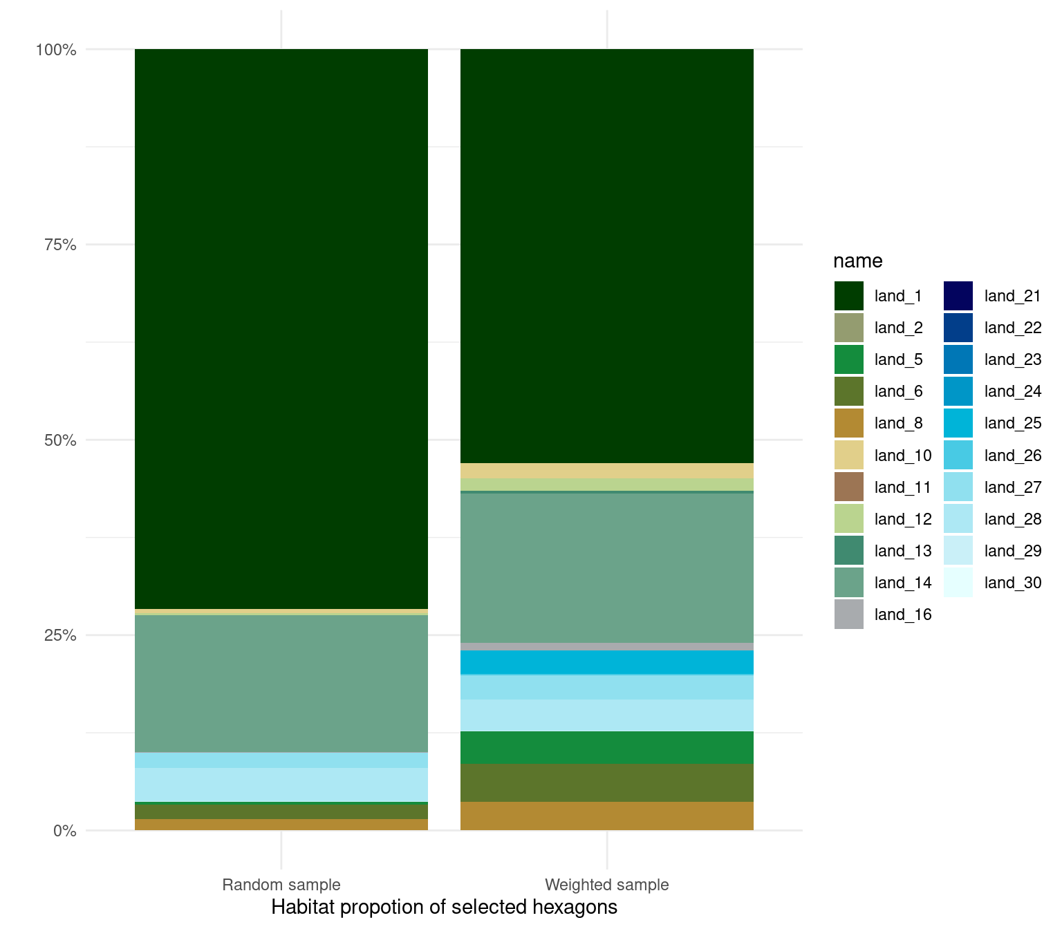
The habitat 1 is the most frequent while the habitat 2 the least. Following the equation above, the inclusion probability of these two habitats are 1.220382e-08 and 7.541478e-05, respectively. This means that although habitat 1 is 6180 times more frequent than habitat 2, they are equally likely to be sampled. For a visual example, we show the relative proportion of habitat from a sample of 10 hexagons with and without inclusion probability Figure 3.2.