7 Secondary sampling unity

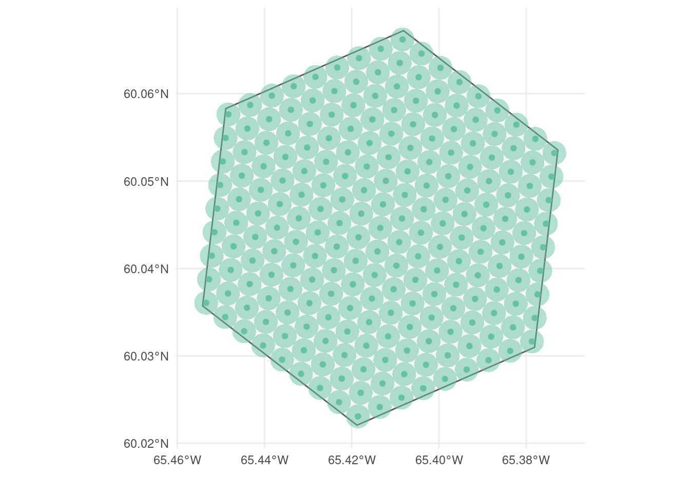
In this section we provide a detail our approach for selecting the Secondary Sampling Units (SSUs). Unlike the PSU sampling, the SSU sampling approach differs significantly from the BOSS design. For each selected hexagon, we create a grid of SSU points spaced 294 meters apart to perfrom the sampling (Figure 7.1). The chosen spacing value was optimized using the Ontario regionalization method to ensure that each hexagon contains an equal number of SSUs.

Figure 7.1: The green dots represent the Secondary Sampling Units (SSUs), which are spatially separated from each other by a distance of 294 meters. A buffer with a diameter of 147 meters was created around each SSU to extract the habitat pixels.

For each SSU point within the PSU, we generate a buffer with a distance of 147 meters. We then extract the habitat pixels to compute the inclusion probability of each SSU point following the same approach used for the PSU (Chapter 3). This process allows us to calculate the habitat inclusion probability and the proportion of non-empty habitats pixels for each SSU hexagon.

The final Step in the process of prepareing the SSU for sampling is to assign a matrix of neighouring SSU points for each focal SSU. This is important because each SSU is classified as available to be sampled in function of its proportion of non-empty habitats pixels, the number of neighbours SSU, and the proportion of non-empty habitats pixels of the neighbours SSUs. Specifically, for a SSU to be available for sampling it must have:

The next step is to assign a matrix of neighboring SSU points for each focal SSU. This is crucial because the availability of each SSU for sampling is determined based on its proportion of non-empty habitat pixels, the number of neighboring SSUs, and the proportion of non-empty habitat pixels of those neighbors. Specifically, to be considered available for sampling, a SSU must meet the following criteria:

Have exactly 6 neighbors (fewer indicates being on the border of the PSU hexagon)
Possess at least 80% non-empty pixels (prop_na = 0.8), similar to the PSU sampling
Have at least 4 out of the 6 neighboring SSUs with at least 80% non-empty pixels

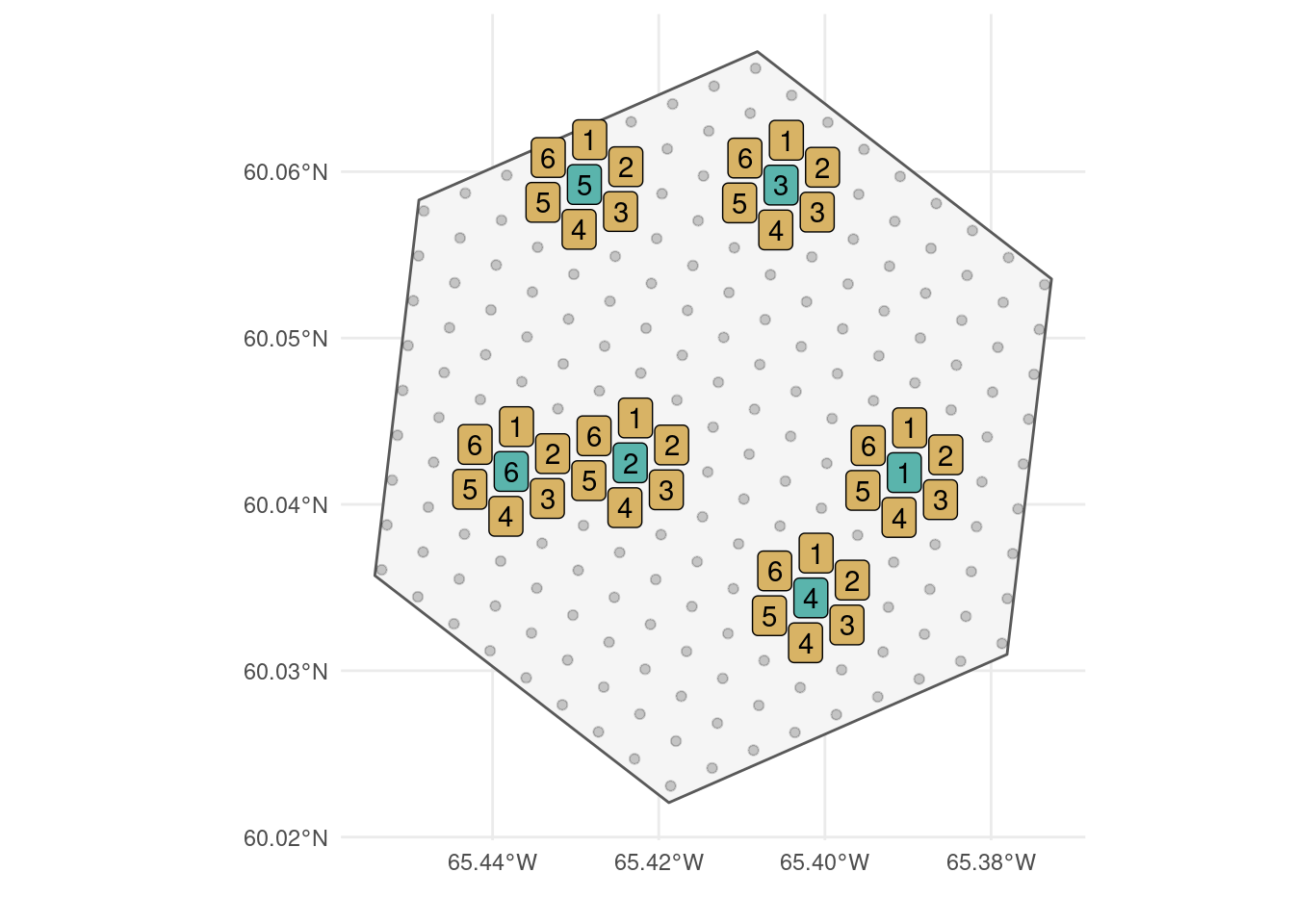
After defining the availability of each SSU, we proceed with a random sampling of SSU points, weighted by their habitat inclusion probability. The SSU sampling is performed sequentially, meaning that for each SSU selected within a PSU hexagon, its six neighbors are automatically marked as unavailable for the next sampling round. This procedure prevents the clustering of SSU samples in a single region. The SSU sampling continues until it reaches the desired SSU sample size (defined by ssu_N), or until there are no more available SSUs remaining. The selected SSU points, along with their respective neighbors, are classified using the \(AB\) code pattern (Figure 7.2). Here, \(A\) represents the SSU sample ID, ranging from 1 to ssu_N, while \(B\) represents the neighbor ID, ranging from 0 to 6. In this pattern, 0 denotes the focal point, while 1 to 6 represent the six neighbors, starting from the North point and moving clockwise.

Figure 7.2: Selected SSU points (green) and their respectice neighboring (yellow).

Once the sampling process is completed, we obtain multiple SSU points for each hexagon from one of the three layers of selected PSU hexagons: main, over, or extra. We export both all SSU points and the selected SSU points for each selected hexagon from the three PSU layers. The export of SSU points follows a similar approach to the export of PSU hexagons. We first export each layer as a separate shapefile, including all ecoregions together, and then create separate shapefiles for each ecoregion. Using the same export parameters utilized in the PSU sampling, the SSU shapefiles will be exported as follows:

/tmp/RtmpHtqxrR/selection
├── allEcoregion
│   ├── SSU-SOQB_ALL_extra-V2023.shp
│   ├── SSU-SOQB_ALL_main-V2023.shp
│   ├── SSU-SOQB_ALL_over-V2023.shp
│   ├── SSU-SOQB_selected_extra-V2023.shp
│   ├── SSU-SOQB_selected_main-V2023.shp
│   └── SSU-SOQB_selected_over-V2023.shp
└── byEcoregion
    ├── ecoregion_101
    │   ├── SSU-SOBQ_eco101_ALL_extra-V2023.shp
    │   ├── SSU-SOBQ_eco101_ALL_main-V2023.shp
    │   ├── SSU-SOBQ_eco101_ALL_over-V2023.shp
    │   ├── SSU-SOBQ_eco101_selected_extra-V2023.shp
    │   ├── SSU-SOBQ_eco101_selected_main-V2023.shp
    │   └── SSU-SOBQ_eco101_selected_over-V2023.shp
    ├── ecoregion_102
    │   ├── SSU-SOBQ_eco102_ALL_extra-V2023.shp
    │   ├── SSU-SOBQ_eco102_ALL_main-V2023.shp
    │   ├── SSU-SOBQ_eco102_ALL_over-V2023.shp
    │   ├── SSU-SOBQ_eco102_selected_extra-V2023.shp
    │   ├── SSU-SOBQ_eco102_selected_main-V2023.shp
    │   └── SSU-SOBQ_eco102_selected_over-V2023.shp
    ├── ecoregion_103
    │   ├── SSU-SOBQ_eco103_ALL_extra-V2023.shp
    │   ├── SSU-SOBQ_eco103_ALL_main-V2023.shp
    │   ├── SSU-SOBQ_eco103_ALL_over-V2023.shp
    │   ├── SSU-SOBQ_eco103_selected_extra-V2023.shp
    │   ├── SSU-SOBQ_eco103_selected_main-V2023.shp
    │   └── SSU-SOBQ_eco103_selected_over-V2023.shp
    └── ecoregion_104
        ├── SSU-SOBQ_eco104_ALL_extra-V2023.shp
        ├── SSU-SOBQ_eco104_ALL_main-V2023.shp
        ├── SSU-SOBQ_eco104_ALL_over-V2023.shp
        ├── SSU-SOBQ_eco104_selected_extra-V2023.shp
        ├── SSU-SOBQ_eco104_selected_main-V2023.shp
        └── SSU-SOBQ_eco104_selected_over-V2023.shp