9  Random effects

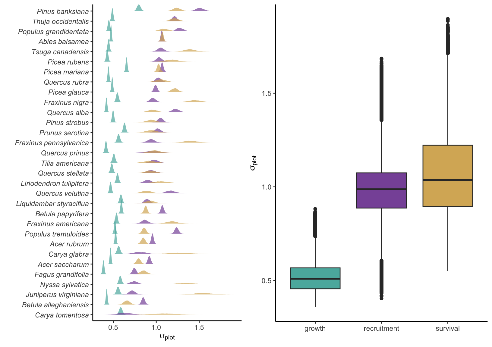
In this section, I discuss the plot random effects affecting growth, survival, and recruitment intercepts. Random effects were used to control for unknown variances grouped within the plot level. For each vital rate and species, the variance among plots was defined by the parameter \(\sigma_{plot}\) where random effects were generated with \(N(0, \sigma_{plot})\).

Variance among plots

Figure 9.1: Posterior distribution of variance in plot random effects across species and vital rates. Note that the parameter is in the scale of the intercept, so it is not comparable between demographic models.

Intercept + random effects

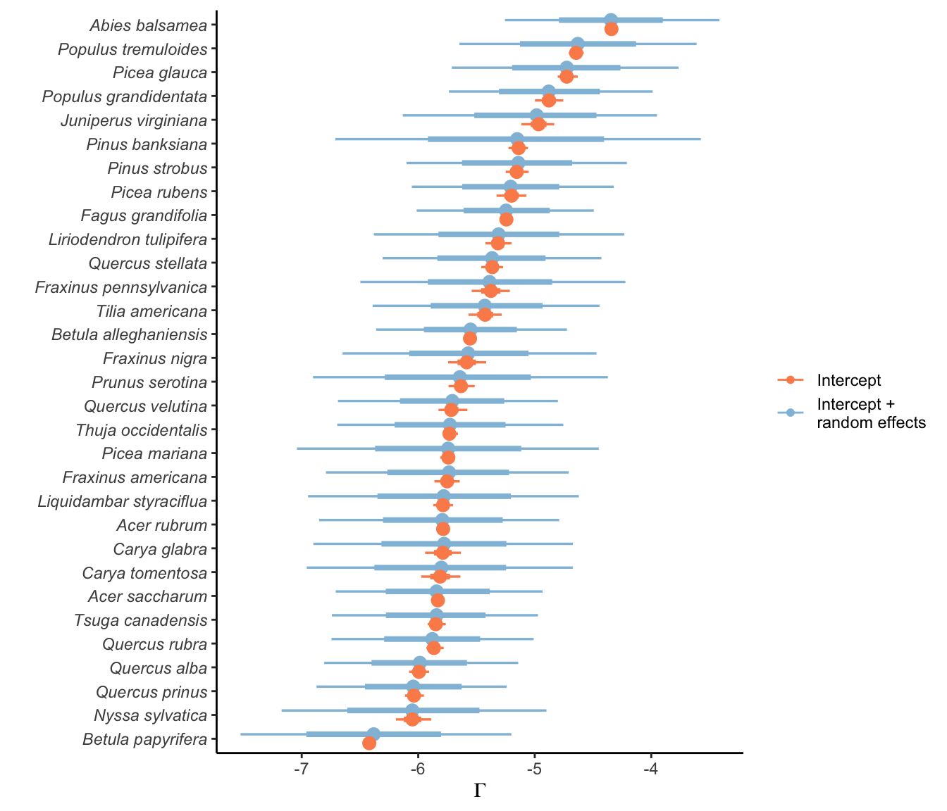
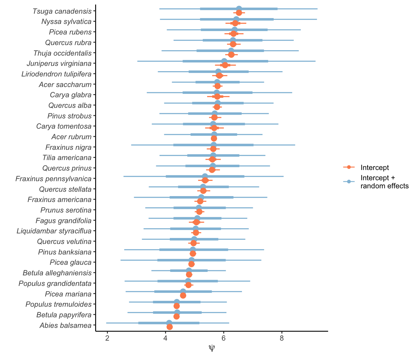
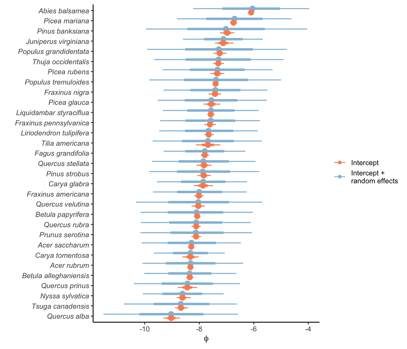
To better understand how plot variation affects growth, survival, and recruitment, the following figures show the intercept distribution for each vital rate and the distribution of a randomly generated offset for plots based on their \(\sigma_{plot}\) parameters.

Growth

Figure 9.2: Posterior distribution of the growth rate intercept (red) and intercept with plot random effects (blue). Plot random effects were randomly generated using a normal distribution with zero mean and the posterior distribution of the among plot variance.

Survival

Figure 9.3: Posterior distribution of the survival intercept (red) and the intercept with plot random effects (blue). Plot random effects were randomly generated using a normal distribution with zero mean and the posterior distribution of the among plot variance.

Recruitment

Figure 9.4: Posterior distribution of the survival intercept (red) and the intercept with plot random effects (blue). Plot random effects were randomly generated using a normal distribution with zero mean and the posterior distribution of the among plot variance.

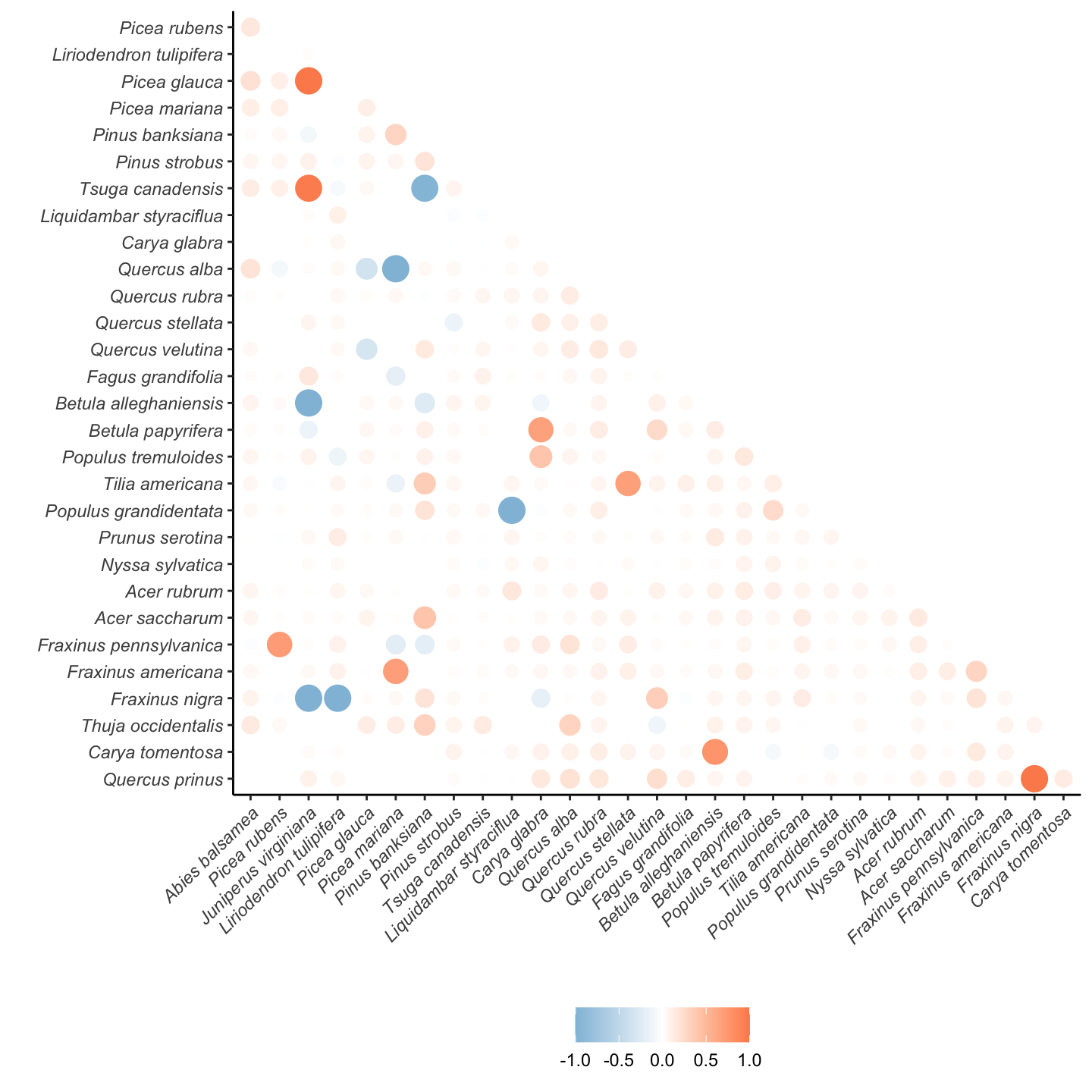
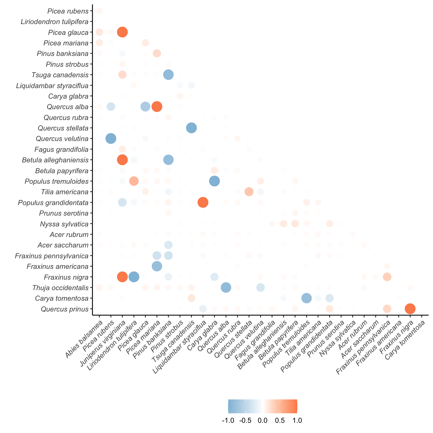
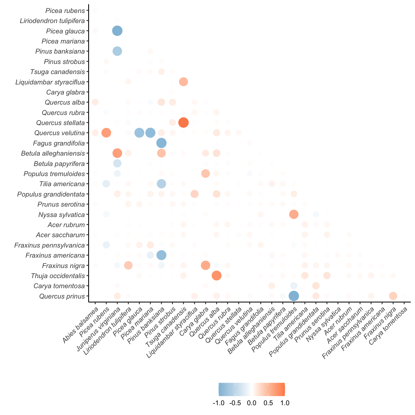
Correlation in Plot Random Effects Among Species

In this section, we compare the correlation among species regarding the plot offset of each demographic model.

Growth

Survival

Recruitment

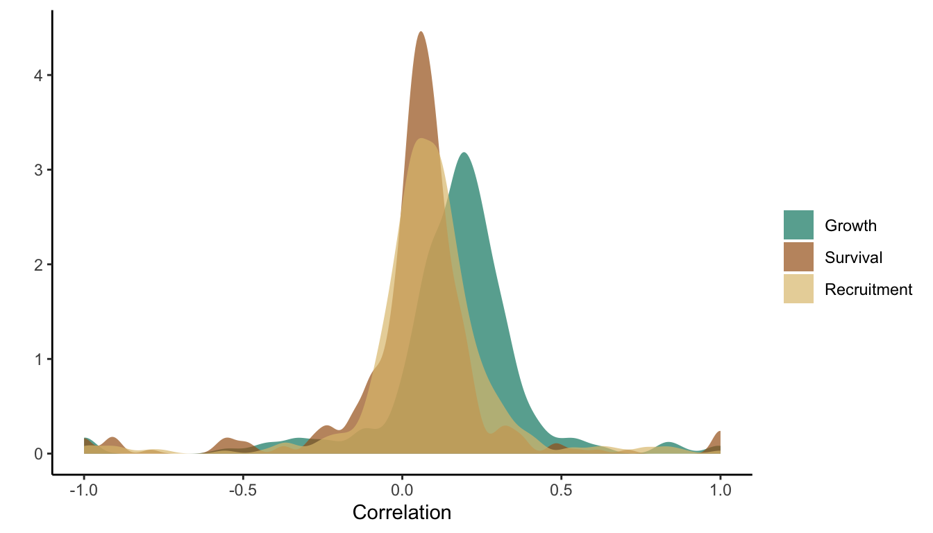
Distribution of the correlation among species par

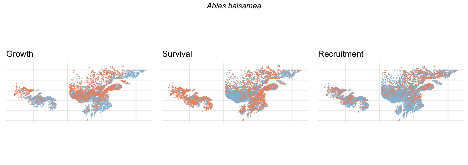
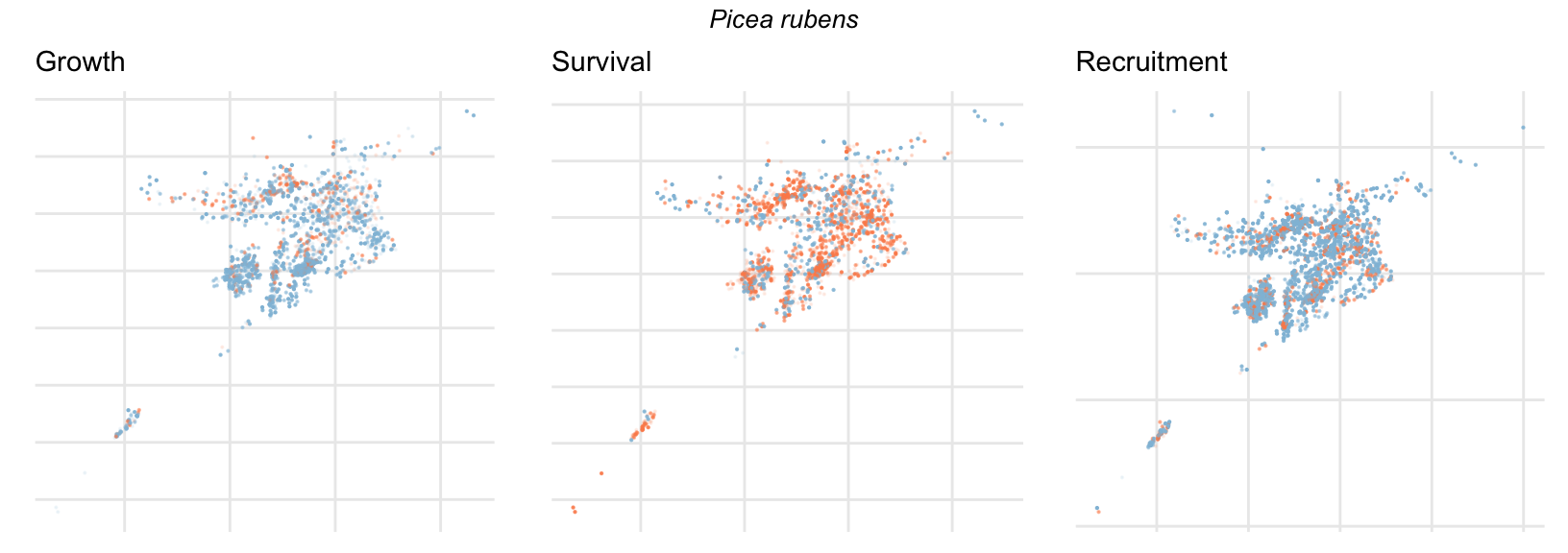
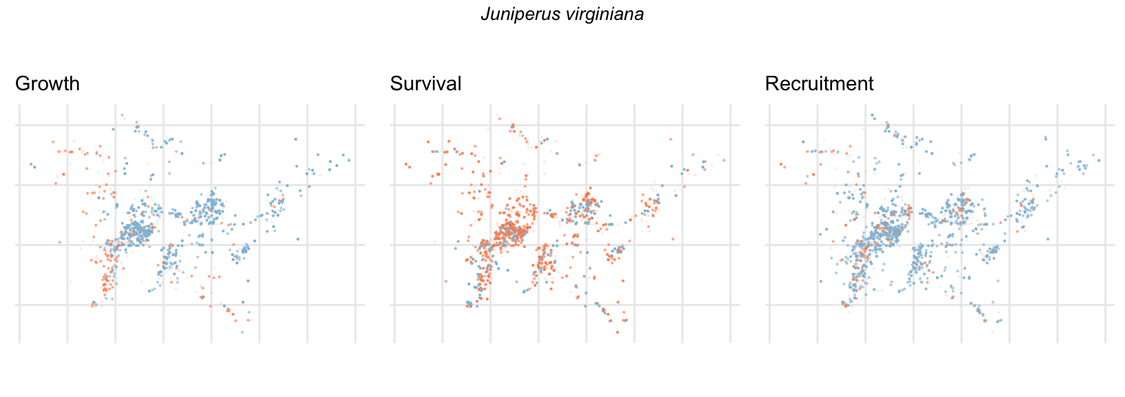
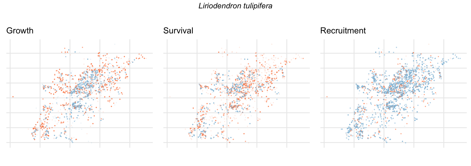
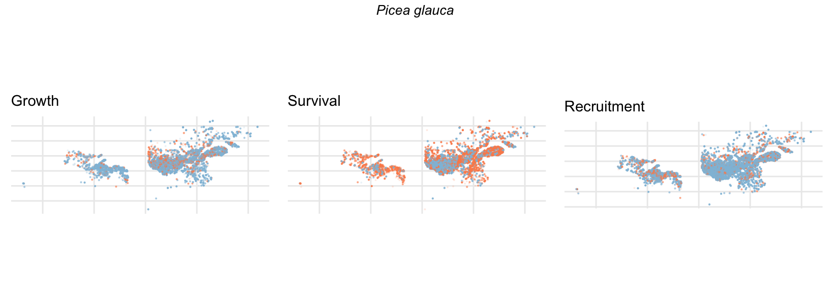
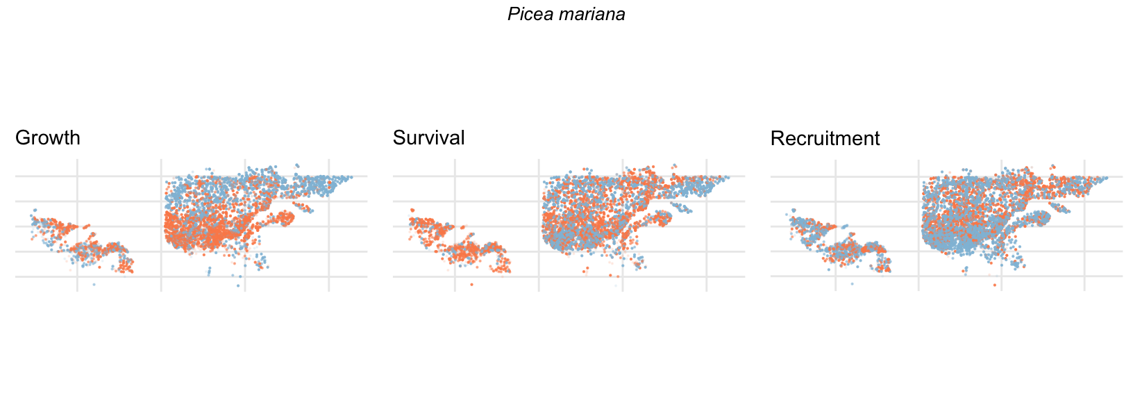
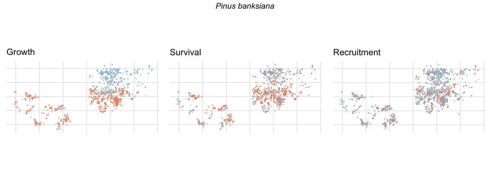
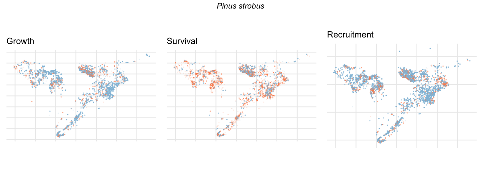
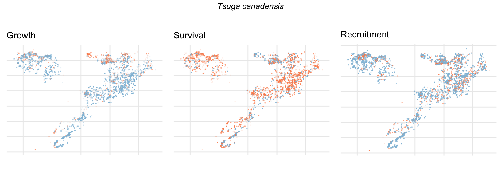
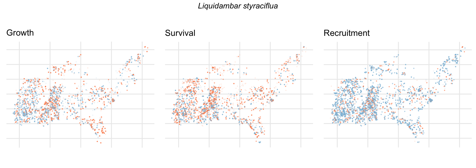
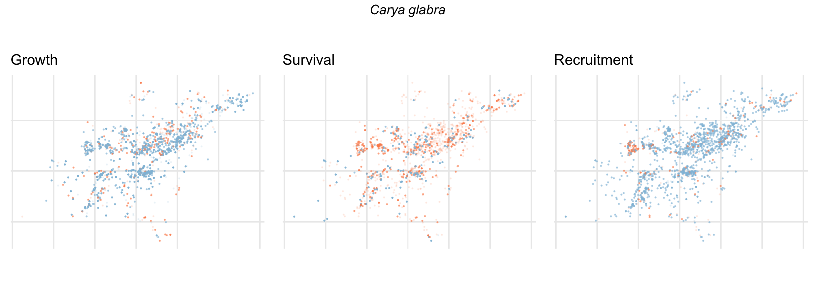
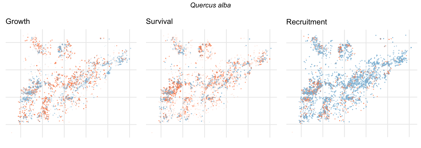
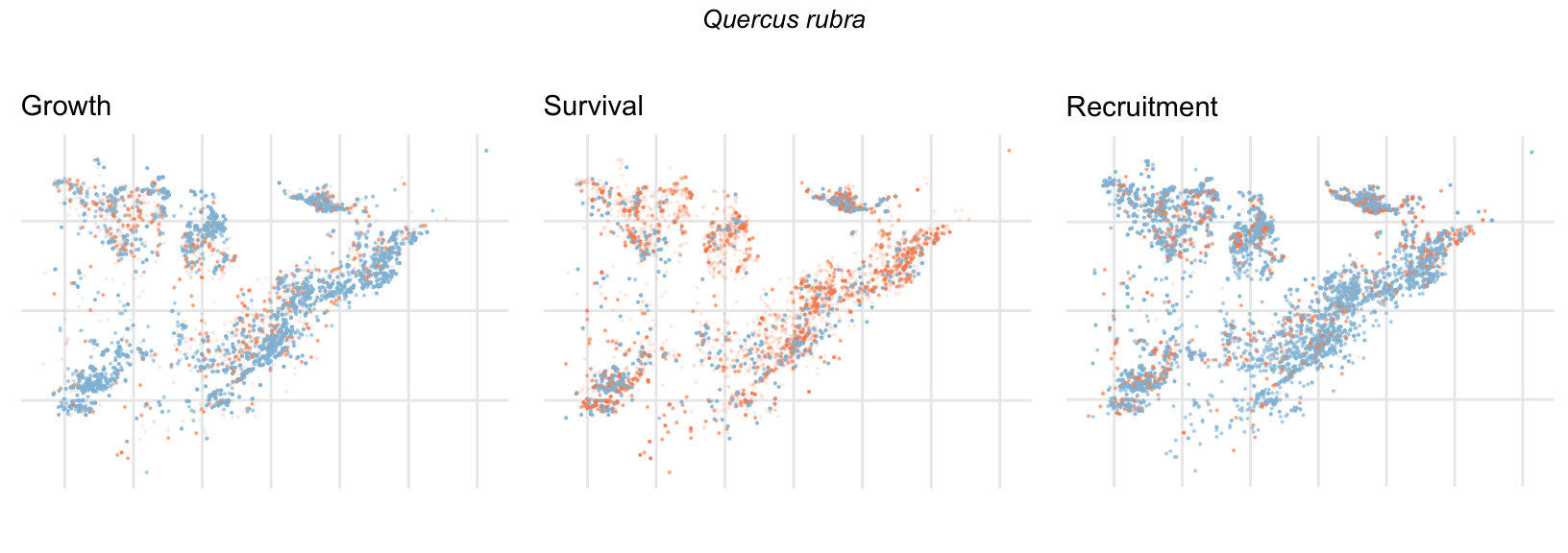
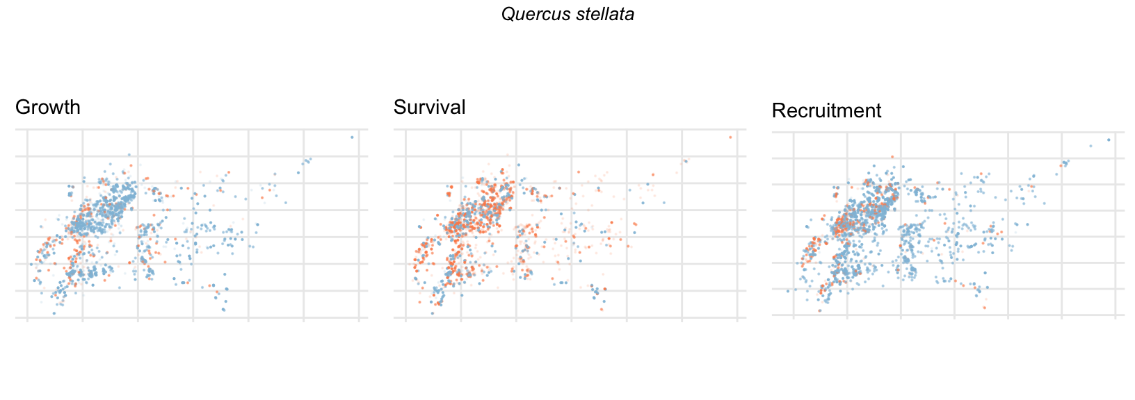
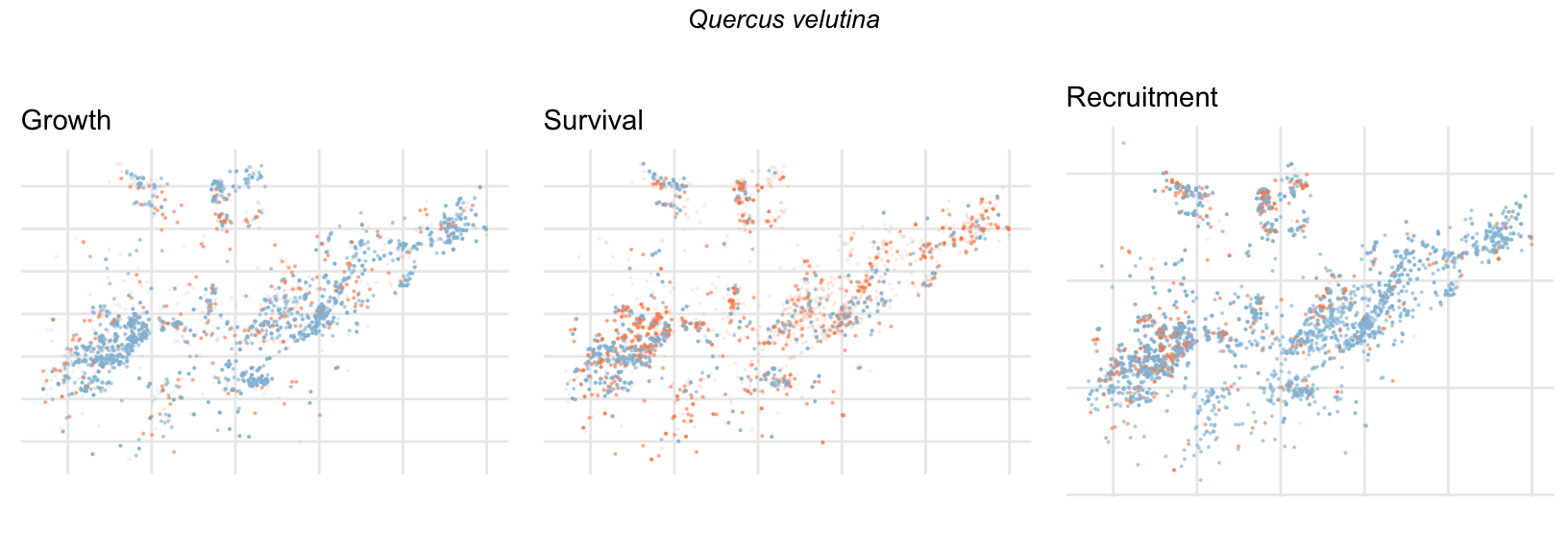
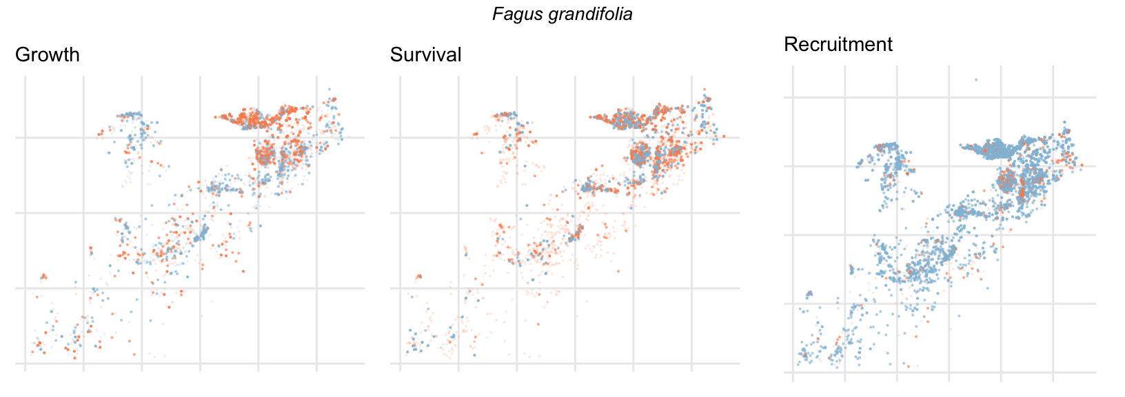
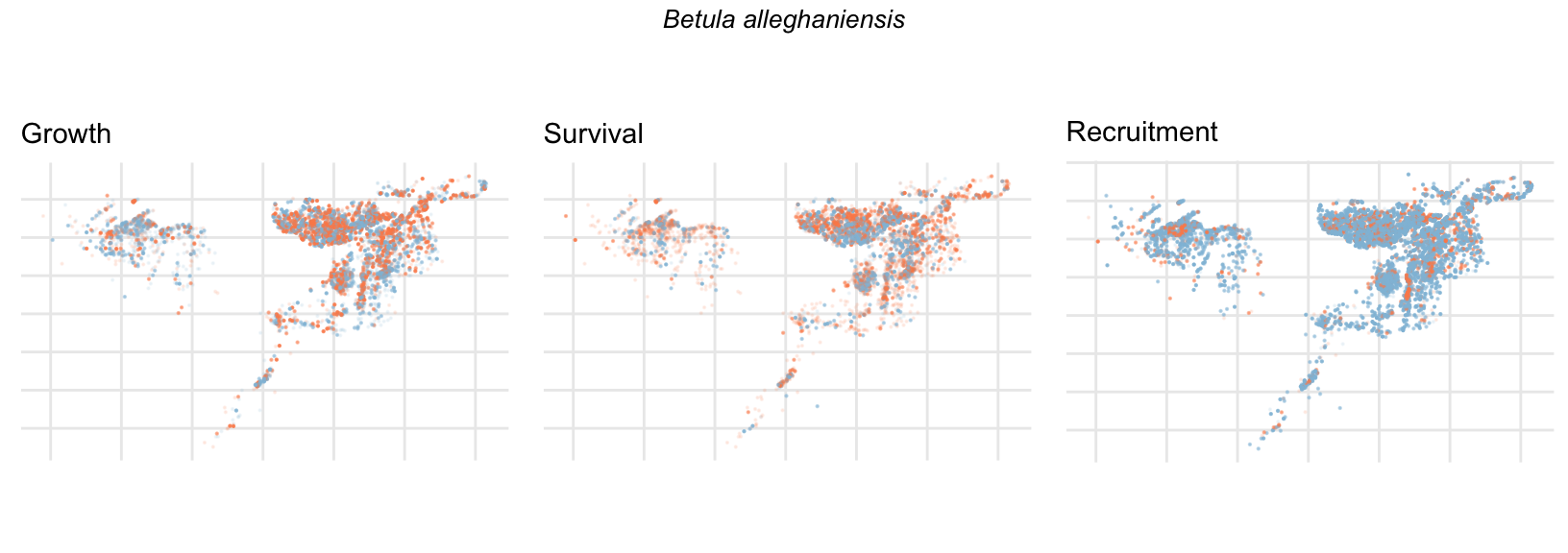
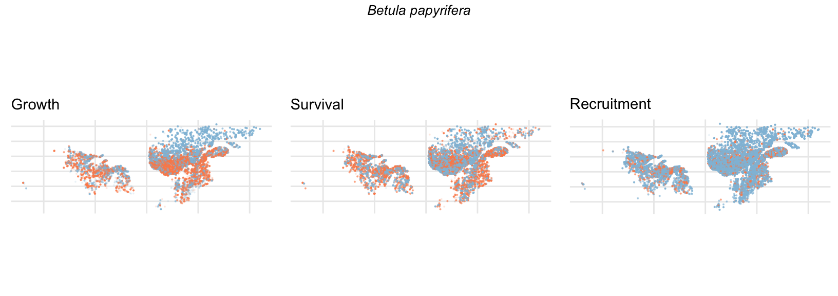
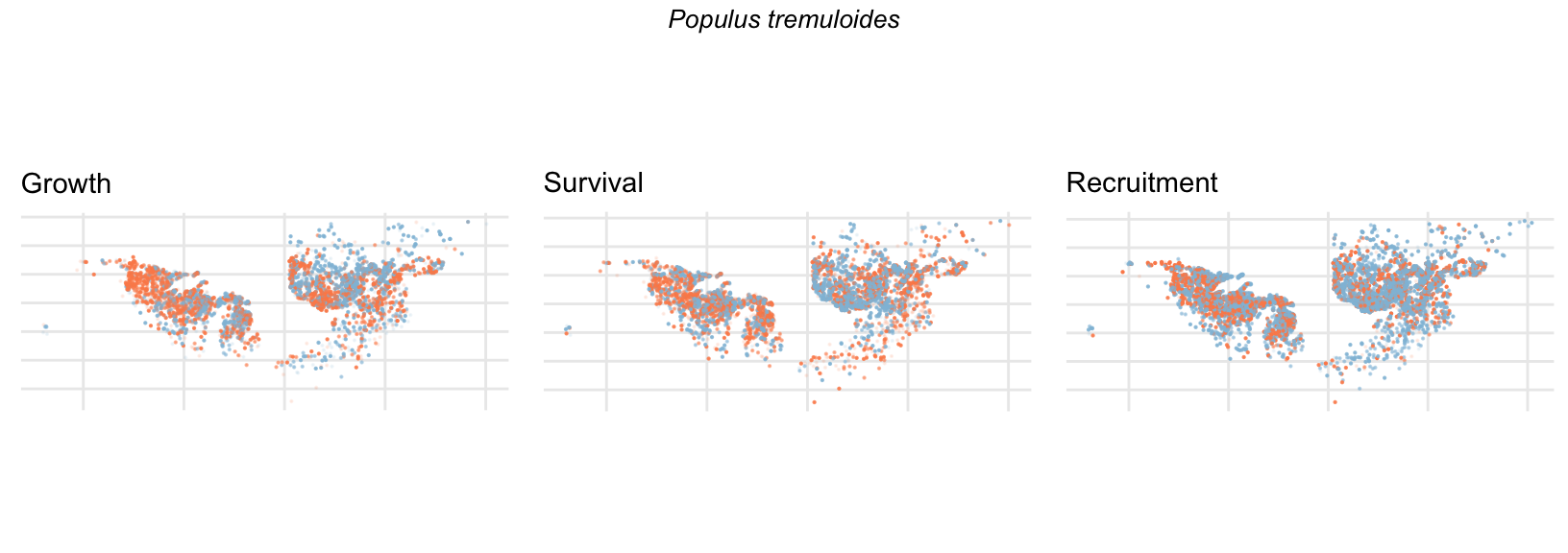
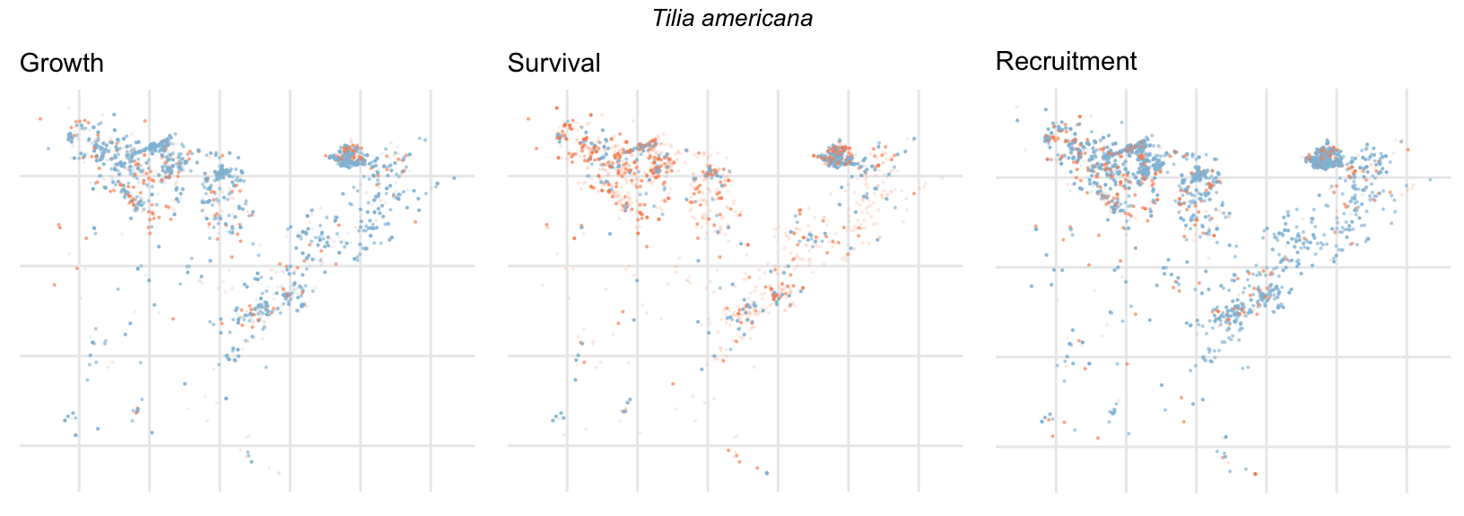
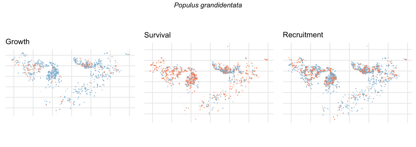
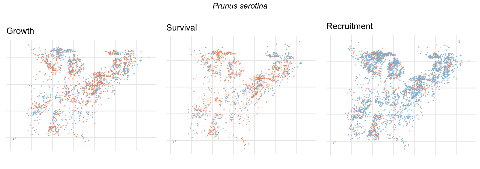
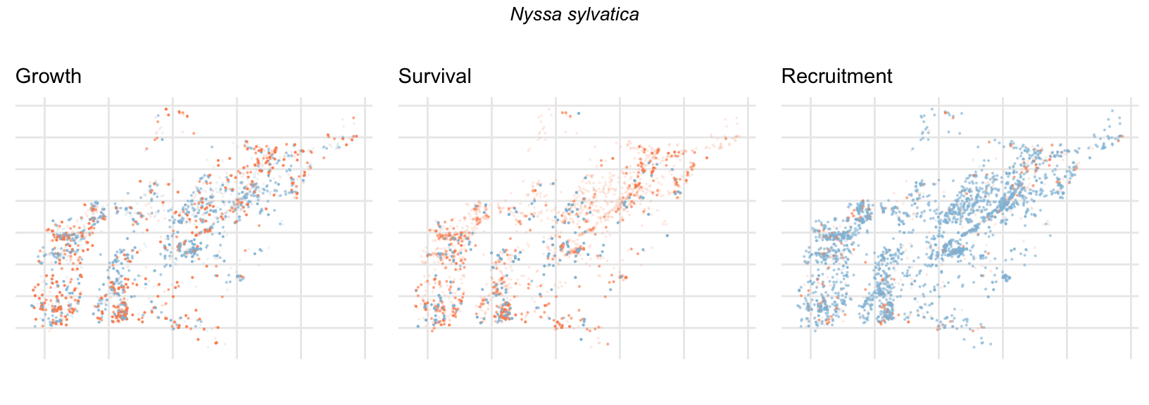
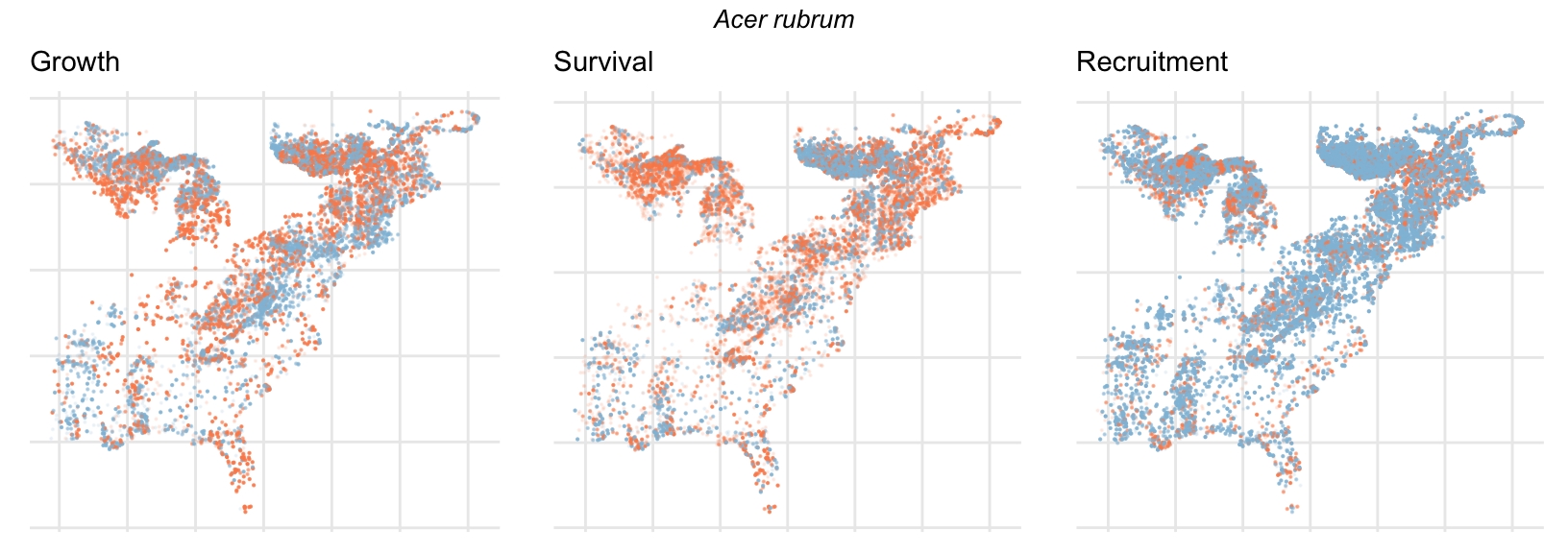
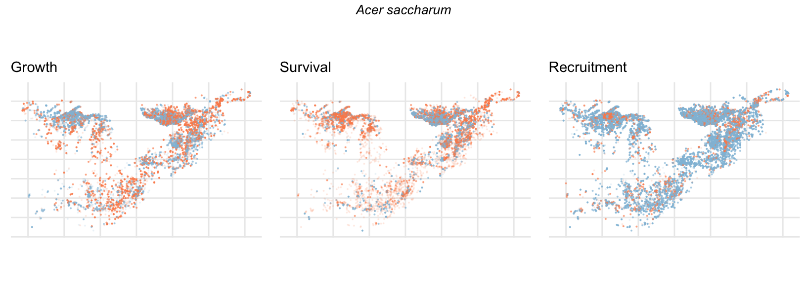
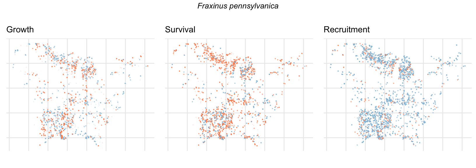
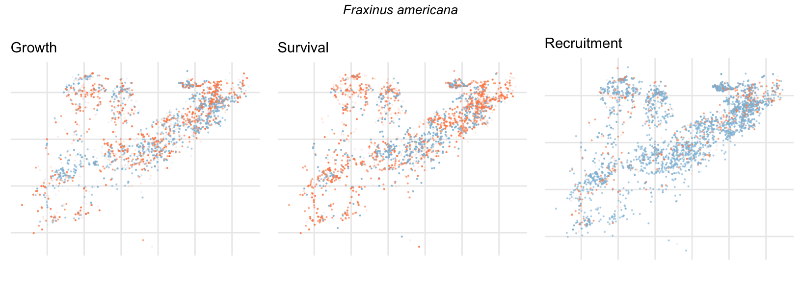
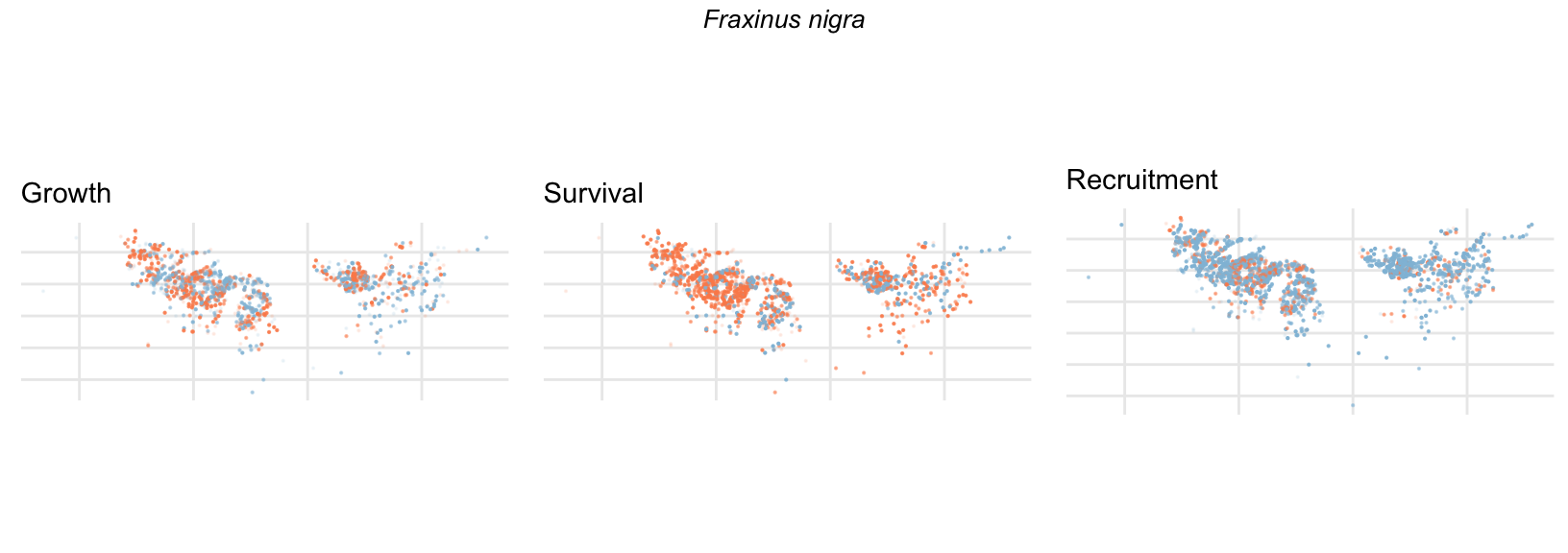
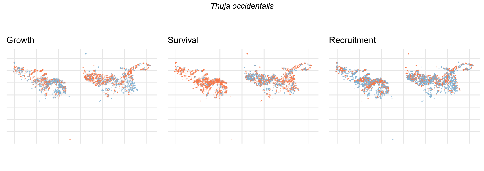
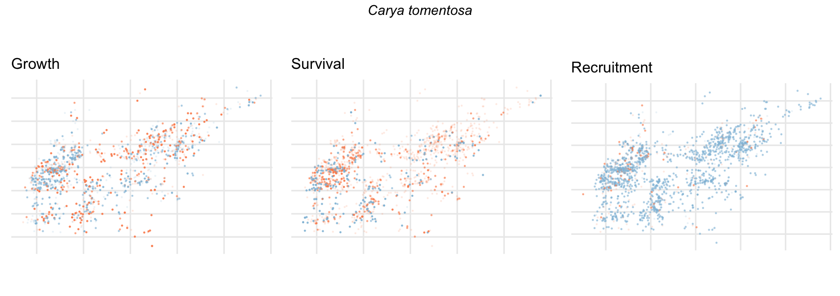
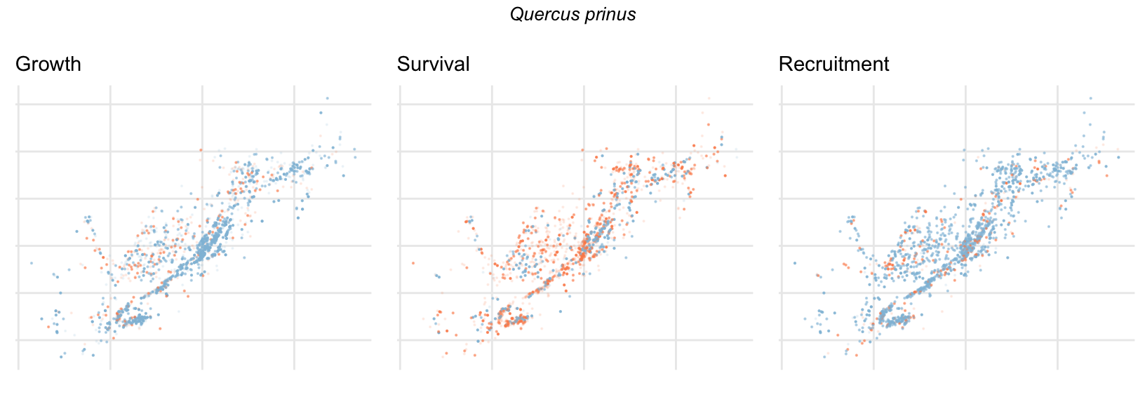
Spatial Distribution of Plot Random Effects

Our modeling approach used a simple hierarchical model that did not explicitly account for the plot identity. However, this section allows us to explore potential spatial structure by visualizing the spatial distribution of the plot’s random effects. As illustrated in the figure below, we categorized the continuous offset values into nine distinct bin classes to aid visualization. To address the issue of overlapping points within the small figures, we use a transparency gradient that allows us to assign more emphasis to plots with higher absolute values.