15 Using the forestIPM package

The forestIPM R package provides a clean R interface for the final Integral Projection Models (IPMs) model and its parameters for the 31 tree species in eastern North America. This guide walks through the complete workflow — from installing the package, setting conditions, to computing population growth rates and projecting a population forward in time, along with some visualization tools.

Setup

Install the package from GitHub:

# install.packages("devtools")
devtools::install_github("willvieira/forestIPM")

library(forestIPM)
library(tidyverse)

We begin by looking which species have fitted parameters and are available in the package:

supported_species()

# A tibble: 31 × 11
   species_id species_name        common_name nom_commun MAT_min MAT_max MAP_min
   <chr>      <chr>               <chr>       <chr>        <dbl>   <dbl>   <dbl>
 1 ABIBAL     Abies balsamea      Balsam fir  Sapin bau…    -5.2     9      433 
 2 ACERUB     Acer rubrum         Red maple   Erable ro…    -1.5    24.7    436 
 3 ACESAC     Acer saccharum      Sugar maple Erable a …    -0.5    16.7    443 
 4 BETALL     Betula alleghanien… Yellow bir… Bouleau j…    -1.4    15.1    529 
 5 BETPAP     Betula papyrifera   White birch Bouleau b…    -5      13.5    395 
 6 CARGLA     Carya glabra        Pignut hic… Caryer gl…     6.3    23.3    631.
 7 CARTOM     Carya tomentosa     Mockernut … Caryer to…     6.7    21.7    589 
 8 FAGGRA     Fagus grandifolia   American b… Hetre a g…    -0.6    20.9    575 
 9 FRAAME     Fraxinus americana  White ash   Frene bla…     0.5    23.3    574 
10 FRANIG     Fraxinus nigra      Black ash   Frene noir     0.1    12.9    320.
# ℹ 21 more rows
# ℹ 4 more variables: MAP_max <dbl>, growth_model <chr>, surv_model <chr>,
#   recruit_model <chr>

Each row lists the species ID (e.g., ABIBAL for Abies balsamea — balsam fir), the common name, nominal french name, the observed climate envelope (MAT and MAP min/max) used during model fitting, and the fitted demographic model from which the parameters are available.

Note

The species_id column is the key you will use throughout the API.

Single-species IPM

In the first example, we will construct a simple plot condition with a single species to compute population growth rate ($\lambda$) for balsam fir (ABIBAL). The forestIPM workflow is built around five constructors and two engines. The constructors capture the ecological context (the stand, the model, the parameters, the climate, and the simulation settings) while the engines run the actual computation. There are two engines, one for computing the punctual $\lambda$ for a given condition, and the other for projecting the dynamics through time.

Step 1: Define the stand with `stand()`

A stand describes a set of interacting individual trees in a given local condition. Specifically, it defined by a collection of trees with their size (mm DBH) and species identity. Note that the minimum DBH is 127 mm - the lower inventory threshold used to fit the models (FIA protocol). We also must define the plot size in which the individuals reside. The stand() function accepts a single data frame object with one row per tree, so it can be easily applied to forest inventory databases. In this example, we will start a small community from scratch with three individuals per two species in a 400 m² plot:

plot_i <- tibble(
  size_mm    = runif(n = 6, 127, 400),
  species_id = c(rep("ABIBAL", 3), rep("ACESAC", 3)),
  plot_size  = 400
)
plot_i

# A tibble: 6 × 3
  size_mm species_id plot_size
    <dbl> <chr>          <dbl>
1    325. ABIBAL           400
2    205. ABIBAL           400
3    207. ABIBAL           400
4    293. ACESAC           400
5    226. ACESAC           400
6    395. ACESAC           400

std <- stand(plot_i)
std

<ipm_stand>  6 trees | 2 species | 400 m2 plot

Important

The IPM is constructed in a way that all species within a plot are interacting with each other. This means that increasing the size of the plot degrades the ecological meaning of the competition. We are using the 400 m² as it’s the size of the FIA protocol.

Step 2: Load the species model with `species_model()`

species_model() reads the fitted Bayesian hierarchical demographic model for one or more species present in the stand. Here we are interested in computing $\lambda$ for the balsam fir:

mod <- species_model("ABIBAL")
mod

<ipm_spModel>  1 species: ABIBAL

Alternatively, you could directly feed the stand() output to the species_model() to automatically defining all species with available parameters to model. In the case a stand have species without available parameters, there are three possibilities the user can assign to the on_missing argument:

"error" (default): abort with a suggestion of the closest valid ID.
"drop": silently remove the unrecognised species; the model runs for the remaining species only.
"static": keep the species as a competitor whose population does not update over time (useful for fixed background competition).

Step 3: Extract parameters with `parameters()`

The parameters() returns one parameter realization from the fitted posterior distribution per mod species. The draw argument determines whether the user wants the "mean" across all 2000 posterior draws, a sampled "random" draw, or a specific draw index (ranging between 1-2000). When draw = "random" a random seed is generated and exported to the object for reproducibility. But the user can also fixed it with the seed argument.

pars <- parameters(mod, draw = "mean")
## Reproducible random draw with fixed seed
# parameters(mod, draw = "random", seed = 42)
## Specific posterior draw (e.g., draw #137)
# parameters(mod, draw = 137)
pars

<ipm_parameters>  draw=mean | 1 species

Plot-level random effects (growth, survival, and recruitment offsets estimated per plot in the hierarchical model) default to zero for all species. To override them use set_random_effects() — see Section 15.5.

Step 4: Set climate conditions with `env_condition()`

env_condition() defines the environmental drivers under which the IPM will run, namely the mean annual temperature and mean annual precipitation:

env <- env_condition(MAT = 8, MAP = 1200)
env

<ipm_env>  MAT=8.0°C  MAP=1200 mm/yr

Further than accepting a numeric scalar (static climate), both arguments also accept a function(t) returning a value for year t (discussed bellow).

Note

If your MAT or MAP values fall outside the range observed during model fitting for any species in the stand, the engines will emit a warning. The valid climate envelope for each species is listed in supported_species() (columns MAT_min, MAT_max, MAP_min, MAP_max).

Step 5: Configure the simulation with `control()`

control() is the central place to set all configuration parameters for both engines. The delta_time is the duration of each timestep in years. In IPMs, it is usually set to 1. The other arguments are either for the project() engine or the discretization approach (both details discussed later). For the lambda() engine, all parameters can be set to defaut.

ctrl <- control()
ctrl

<ipm_control>  100 years | dt=1.0 | store_every=1 | bin_width=1 | lambda=yes | progress=yes | integration=gauss-legendre

Step 6: Compute population growth rate with `lambda()`

Once all constructors are defined, we can approximate the population growth rate ($\lambda$) for a given condition:

lam <- lambda(mod, pars, std, env, ctrl)
lam

<ipm_lambda>  draw=mean
  ABIBAL: 1.4227

Multi-species IPM through time

Different from the lambda() engine, project() advances the population forward in time, updating the kernel at every timestep to account for the current size distribution (density-dependent dynamics). This engine also depends on the five constructors. Here we will the same conditions set to run the single species IPM.

If we plugged all predefined conditions into the project() engine, it would return an error stating that there are species in the std which do not have its parameters in pars. Indeed, project() needs parameters for all species present in the stand, and when there is no parameter available, we have to explicit handle it with the on_missing argument in species_model(). To avoid the error, we will first update the mod and pars objects to also account for the sugar maple along with the balsam fir:

(mod <- species_model(std))

<ipm_spModel>  2 species: ABIBAL, ACESAC

(pars <- parameters(mod, draw = "random"))

<ipm_parameters>  draw=random (id=712) seed=2127826300 | 2 species

As we will project population over time, let’s take the opportunity to see how we can set a dynamic environment. We will simulate a 4°C degree increase for the first 100 year and keep it constant for the remaining years as follows:

temp_warm <- function(t) {
  if(t <= 100) {
    return( 8 + (4/100) * t)
  }else{
    return( 8 + 4 )
  }
}

env <- env_condition(MAT = temp_warm, MAP = 1200)
env

<ipm_env>  MAT=<function>  MAP=1200 mm/yr

Before running projection, we can take a look in the available controls for this engine:

ctrl <- control(
  delta_time = 1,
  years = 300,            # only used in `project()`
  store_every = 1,        # only used in `project()`
  compute_lambda = TRUE,  # only used in `project()`
  progress = FALSE,       # only used in `project()`
  integration_method = "gauss-legendre",
  n_gl = 200L,            # for integration = "gauss-legendre"
  bin_width = 1           # for integration = "midpoint"
)

years define the total simulation length and store_every the steps in which it will save population summaries and lambda computation if compute_lambda = TRUE. The remaining three arguments can be set to default given the Gauss-Legendre Quadrature is both more efficient and mathematically more precise than the midpoint rule to numerically integrate the Kernel.

Now that we have set conditions, we can simulate the community dynamics for the specified time frame:

proj <- project(mod, pars, std, env, ctrl)
summary(proj)

<ipm_projection> summary
  Species (2): ABIBAL, ACESAC
  Timesteps stored: 300 (years 1 to 300)
  Final timestep per species:
    ABIBAL: lambda=1.0001, n_trees=153
    ACESAC: lambda=0.9985, n_trees=42
  Parameters: random (id=712, seed=2127826300)
  Climate: MAT=function(t)  MAP=1200 mm/yr

Visualizing project results with `plot()`

Calling plot() on a projection renders diagnostic panels. Use type to select a specific panel:

type — character or NULL. Selects which panel to render. Options:
- NULL (default): all four panels in sequence.
- "lambda": population growth rate $\lambda$ over time.
- "pop_size": total population size (N) over time.
- "size_dist": size distribution at a single timestep.
- "lambda_vs_n": phase portrait of $\lambda$ vs N.
timestep — integer or NULL. Only applies to type = "size_dist". The stored year to plot (must be one of proj$years). Defaults to the last stored timestep.

Lambda trajectory

plot(proj, type = "lambda")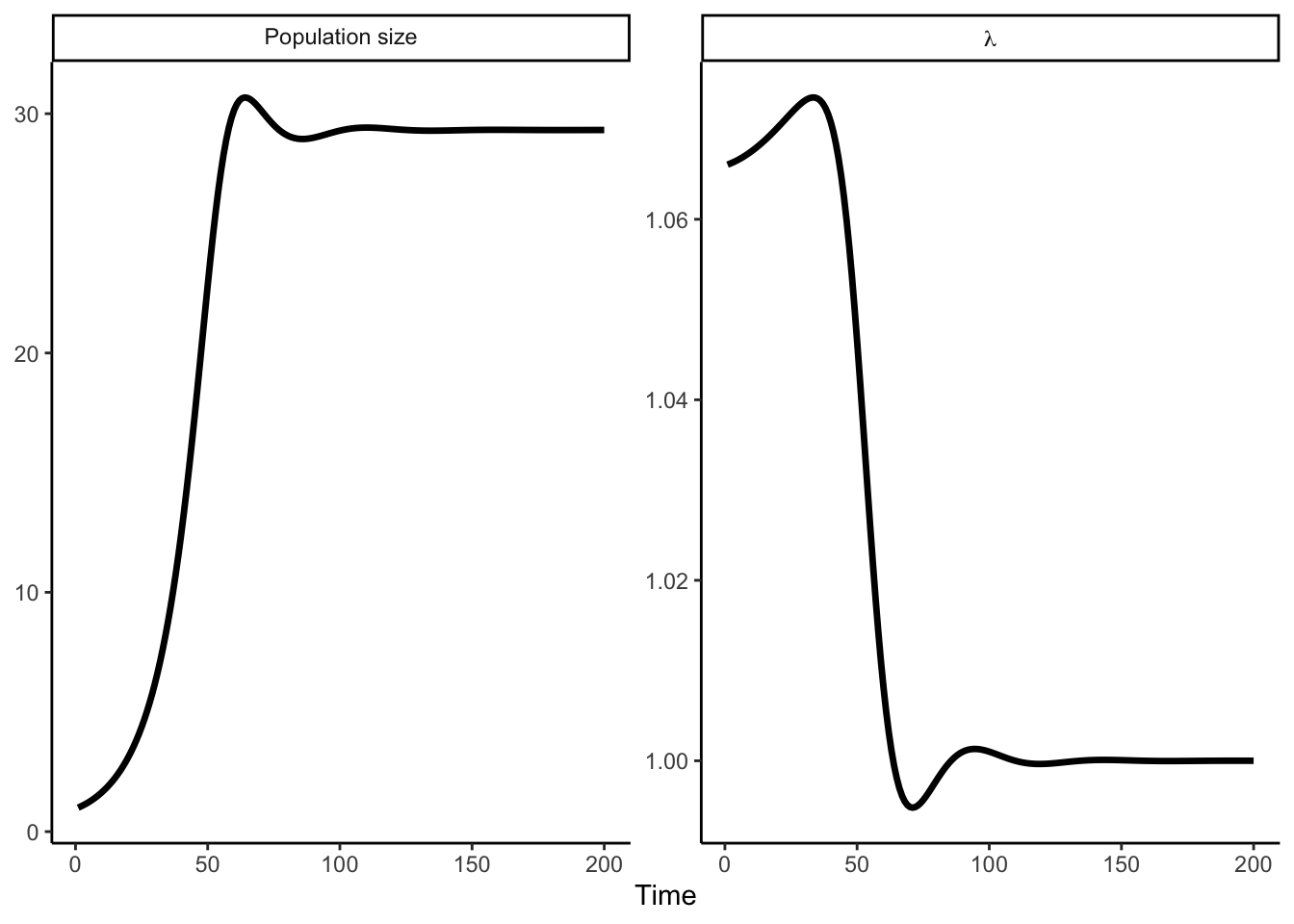

Figure 15.1: Population growth rate ($\lambda$) over time. Values above 1 indicate growth; below 1 indicate decline.

$\lambda$ starts above 1 when the stand is sparse (low intraspecific competition) and converges toward 1 as the population reaches carrying capacity.

Population size trajectory

plot(proj, type = "pop_size")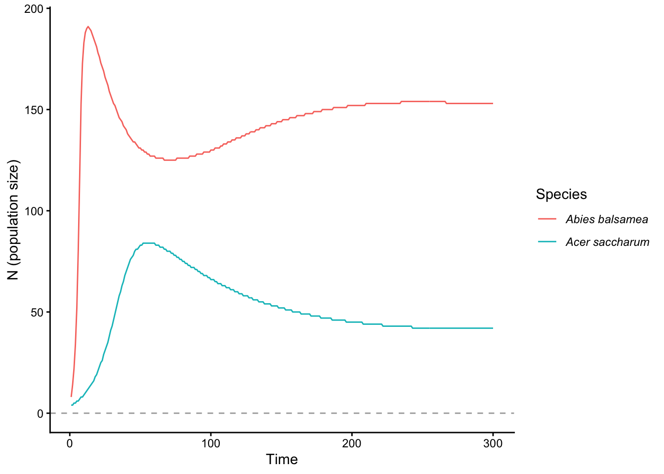

Figure 15.2: Total population size (N, number of individuals) over time.

Size distribution over time

plot(proj, type = "size_dist")           # default: last stored timestep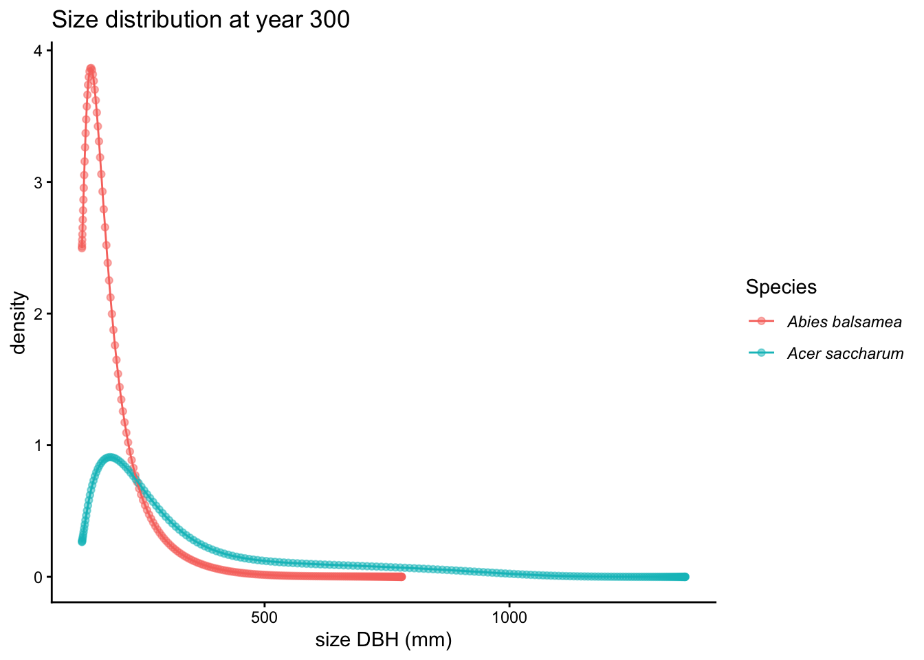

Figure 15.3: Size distribution of *Abies balsamea* and *Acer saccharum* at the last time step.

Use timestep to inspect an earlier snapshot:

plot(proj, type = "size_dist", timestep = 10)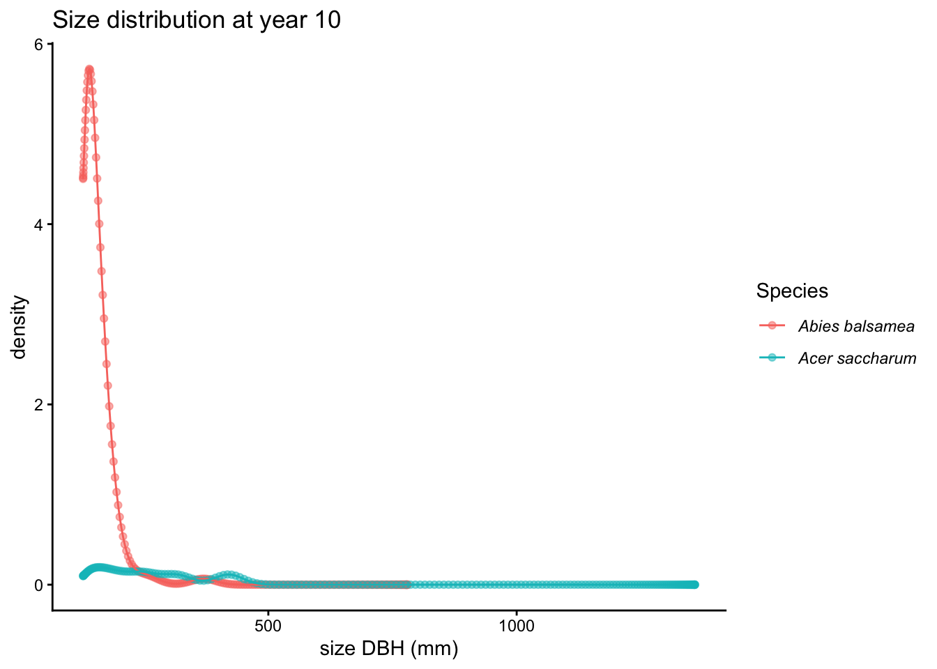

Figure 15.4: Size distribution at year 10.

Lambda vs population size

plot(proj, type = "lambda_vs_n")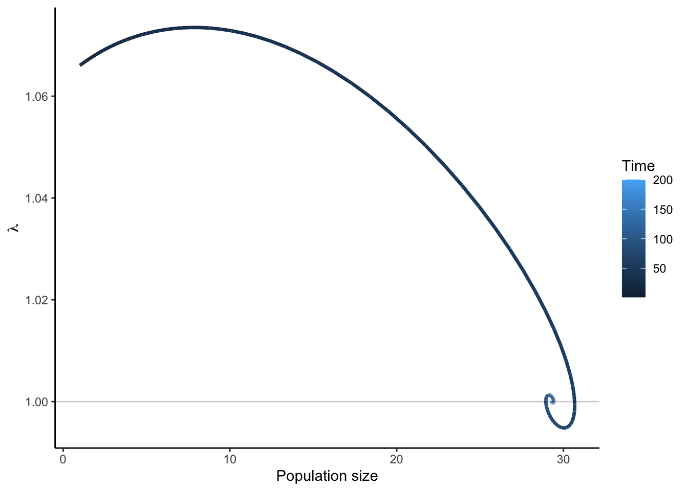

Figure 15.5: Phase portrait of $\lambda$ against total population size. Colour gradient indicates time.

This phase portrait shows the classic density-dependent trajectory: $\lambda$ is high when population size is low and declines as intraspecific competition intensifies, eventually stabilising near $\lambda = 1$.

Plot-level random effects

The demographic models are hierarchical: each plot has random intercepts for growth, survival, and recruitment that shift the vital rates above or below the population mean. By default, parameters() sets all random effects to zero (population-mean predictions).

To apply plot-specific random effects — for example if you have inventory data from a known plot — use set_random_effects():

# Apply the same offsets to all species in pars
pars_re <- set_random_effects(
  pars,
  values = c(0.1, -0.05, 0.0)   # growth, survival, recruitment offsets
)

# Or apply species-specific offsets via a named list
pars_re2 <- set_random_effects(
  pars,
  values = list(
    ABIBAL = c(0.1, -0.05, 0.0)
  )
)

Arguments:

pars — an ipm_parameters object.
values — either a numeric(3) vector applied to the species listed in species, or a named list keyed by species ID where each element is a numeric(3) vector.
species — character vector of species IDs. Used only when values is a numeric vector. If NULL (default), the offsets are applied to all species in pars.

The three offsets correspond to the random intercepts in the growth, survival, and recruitment sub-models respectively.

Reproducibility

Every ipm_lambda and ipm_projection object carries a $conditions record that captures the exact parameter draw, seed, and climate values used to produce the result. This makes any analysis self-documenting — you can always recover the exact inputs from the output alone.

# The conditions record is embedded in the projection object
names(proj$conditions)

[1] "on_missing" "stand"      "env"        "pars"       "ctrl"

ROADMAP

The next developpement phase can include

random effects cloud accecibility
smooth gaussian model to predict random effects for any location
new functionality to fit and evaluate Stan model for new speceis
expand to include dynamic modifiers (immigration, fire/insect disturbance, forest management, etc)

Setup

Single-species IPM

Step 1: Define the stand with stand()

Step 2: Load the species model with species_model()

Step 3: Extract parameters with parameters()

Step 4: Set climate conditions with env_condition()

Step 5: Configure the simulation with control()

Step 6: Compute population growth rate with lambda()

Multi-species IPM through time

Visualizing project results with plot()

Lambda trajectory

Population size trajectory

Size distribution over time

Lambda vs population size

Plot-level random effects

Reproducibility

ROADMAP

Step 1: Define the stand with `stand()`

Step 2: Load the species model with `species_model()`

Step 3: Extract parameters with `parameters()`

Step 4: Set climate conditions with `env_condition()`

Step 5: Configure the simulation with `control()`

Step 6: Compute population growth rate with `lambda()`

Visualizing project results with `plot()`