21 Suitable probability
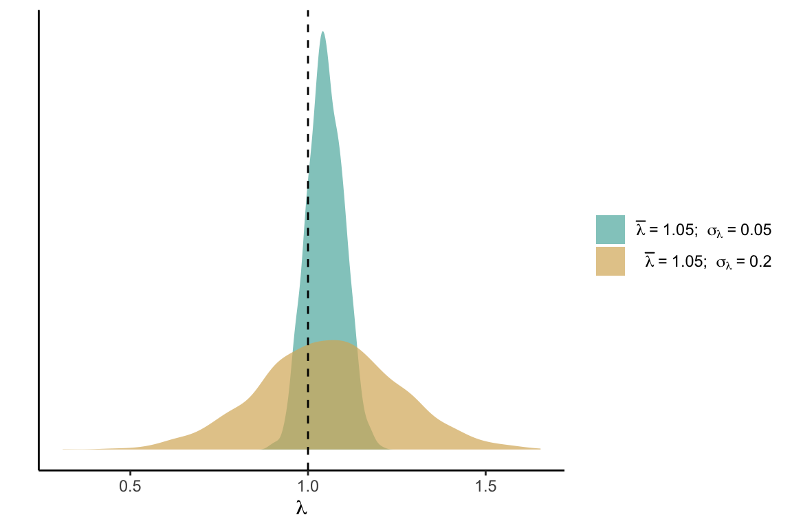
In this section, we discuss the concept and application of suitable probability derived from the stochastic population growth rate in the IPM. The variability in the population growth rate (\(\lambda\)) arises from both environmental stochasticity and parametric uncertainty. The former combines spatial and temporal variation in the climate (mean annual temperature and precipitation) and variation in the strength of competition for light. The latter combines model uncertainty at the individual level for the growth, survival, and recruitment models, along with the spatial heterogeneity determined by the variance of these demographic models among local populations (plot level variability). The inherent demographic uncertainty and environmental stochasticity introduce variance into \(\lambda\), and the strength of this variance directly influences the suitable probability, especially for populations with lower performance or density (Holt et al. 2005). To illustrate the concept, consider two populations with equal mean growth rates (\(\overline{\lambda}\)) but varying standard deviations (\(\sigma_\lambda\)). We define suitable probability as the area under the distribution for \(\lambda \geq 1\) Figure 21.1.
To estimate suitable probability, we first determine the cumulative distribution function, \(F(x)\), from the generic probability density function, \(log(\lambda) = f(t)\), as follows:
\[ F_{\lambda}(x) = P(\lambda \le x) = \int_{-\infty}^{0} f(t)dt \tag{21.1}\]
This function represents the cumulative distribution from \(-\infty\) to \(x\). Subsequently, we define the suitable probability (\(\Lambda\)) as the inverse of the cumulative distribution function for \(x = 1\):
\[ \Lambda = 1 - F_{\lambda}(1) \tag{21.2}\]
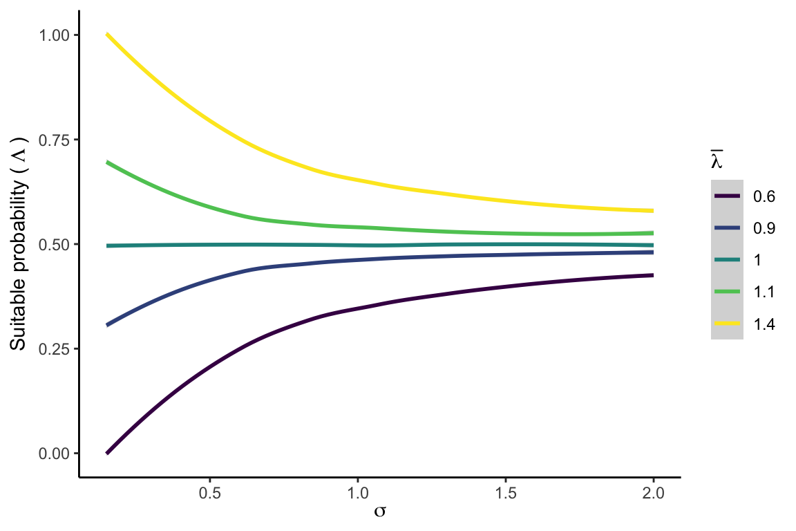
Figure 21.2 illustrates the relationship between \(\lambda\) variability and \(\Lambda\). The higher the variability around \(\lambda\), the more blurred the mean difference between two populations will become. Increasing variance tends to reduce suitable probability when the population growth rate is below 1.
Simulating the effect of demographic uncertainty and environmental stochasticity
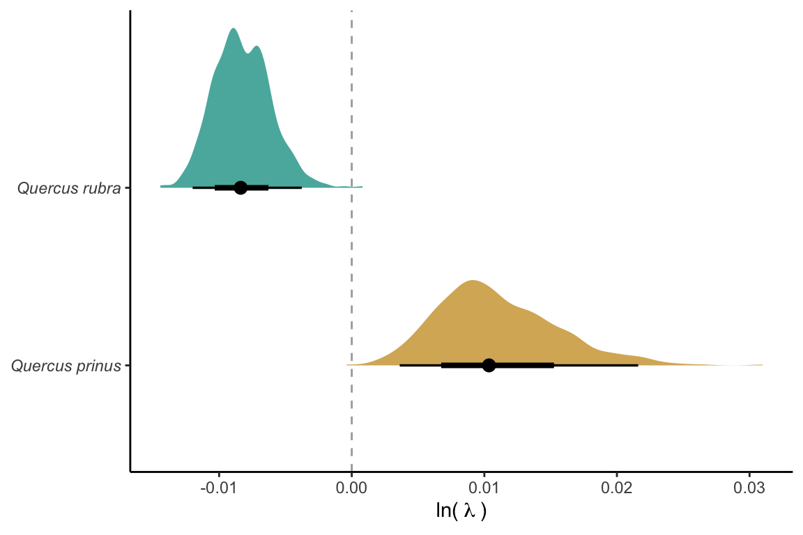
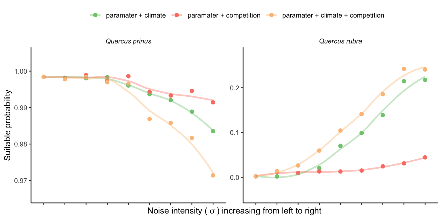
In this section, we investigate how increasing the uncertainty of parameters and the variability of covariates affects the suitable probability. We selected two species, Quercus prinus and Quercus rubra, with an average \(\lambda\) close to 1, and were sensitive to competition and climate covariates. We set these species to conditions with population growth rates closest to 1 but with different average values (lower for Q. rubra and higher for Q. prinus) for comparison Figure 21.3.
We used the same 500 parameter draws from the posterior distribution defined in the sensitivity analysis section (Chapter 18). We conducted four simulations to understand the cumulative impact of demographic uncertainty, environmental, and environmentally induced competition stochasticity. First, we quantified suitable probability under demographic uncertainty using the posterior parameter distribution while keeping the covariates at their mean conditions, effectively simulating zero noise from the covariates. Subsequently, we introduced environmental stochasticity and demographic uncertainty by adding noise to the mean temperature conditions. Similarly, we introduced noise to the mean basal area of heterospecific individuals while keeping temperature constant at the mean. Finally, we added all sources of variability together, encompassing demographic, environmental, and environmentally induced competition variability. We increased the standard deviation (SD) for temperature from 0.1 to 1.5, and for basal area, SD increased from 1 to 8.
Figure 21.4 shows the changes in \(\lambda\) variability with increased variability of the covariates. The panels illustrate the effect of climate stochasticity, competition stochasticity, and both combined factors.
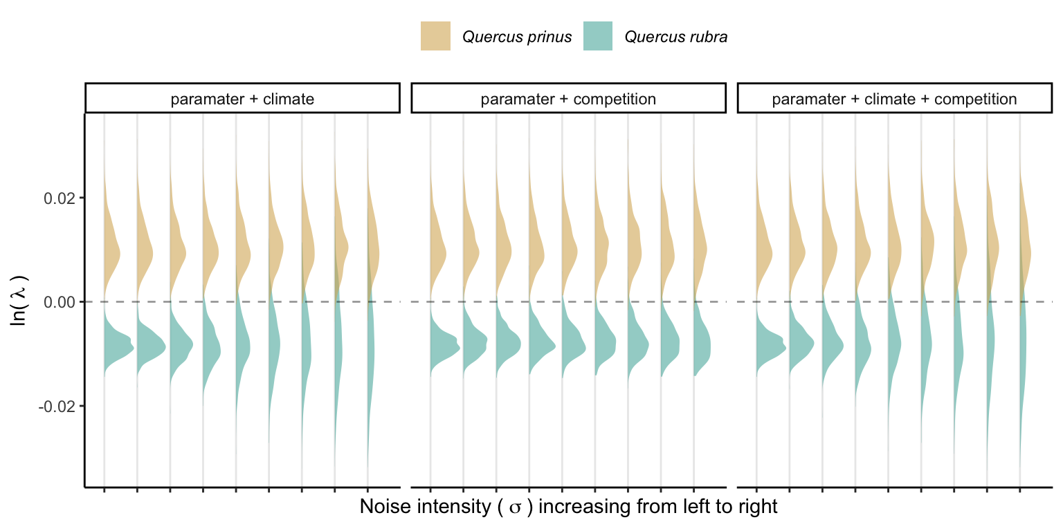
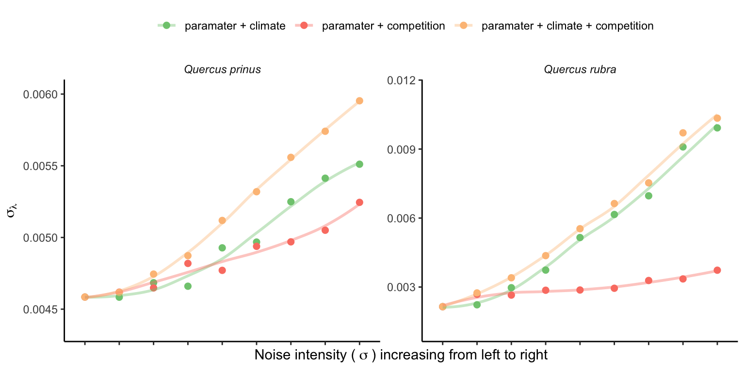
Figure 21.4 and Figure 21.5 highlight that increased noise around the average covariate conditions leads to higher variability in \(\lambda\). It is important to note that the y-scale on the panels in Figure 21.5 is standardized, showing a higher \(\lambda\) variability for Q. rubra compared to Q. prinus. This suggests that climate and competition are more significant predictors for all vital rates of Q. rubra compared to Q. prinus. In summary, higher variability in covariates will likely increase the variability in \(\lambda\), proportional to the covariate sensitivity.
Once we determine the uncertainty in \(\lambda\), we can calculate population-level suitable probability using the cumulative distribution function \(F(\lambda)\). Figure 21.6 illustrates how suitable probability increases for Q. prinus and decreases for Q. rubra with increased variability of covariates.
Objective
This exploration shows that parametric uncertainty and environmental stochasticity can increase \(\lambda\) variability and change suitable probability. In this chapter, we want to assess the effect of spatio-temporal environmental variability and demographic uncertainty on the suitable probability of each species. Specifically, we aim to model how the suitable probability changes from the center toward the cold and hot temperature range distribution. By having the suitable probability varying across the temperature range, we can predict the effect of climate and competition, along with environmental variability and model uncertainty, on the range limits of forest trees. This new approach allows us to test whether species interaction (here competition) can set range limits while accounting for the uncertainty of the estimations. We conclude this study with a novel theory that uses suitable probability to establish the link between individual demographic rates and metapopulation dynamics.
Methods
Sources of population growth rate (\(\lambda\)) variability
The estimation of \(\lambda\) occurs at the local population scale, specifically at the plot level in our study. Within a given geographic location, such as a specific latitude where several plots are located, the variance of \(\lambda\) among those plots arises from spatio-temporal variations in both climate and competition covariates. For instance, climate stochasticity introduces noise in annual temperature and precipitation, leading to environmental variations. Similarly, even with identical climate conditions, two locations can exhibit different community abundance and composition, resulting in variability in the strength of competition. Beyond these spatio-temporal environmentally-induced variations, \(\lambda\) can still vary due to model uncertainty.
In our study, demographic models track uncertainty at two complementary scales: individual and plot levels. At the individual level, plots with the same climate and competition conditions may have different \(\lambda\) values due to the uncertainty in the demographic models. Similarly, even with the same environmental conditions and averaged parameter values (eliminating demographic uncertainty at the individual level), two plots can still yield different \(\lambda\) values due to the spatial uncertainty of each demographic model assigned among plots through the random effects. Therefore, variability in the population growth rate can arise from spatio-temporal variations in both the environment and the parameters.
Modeling suitable probability
We can evaluate the suitable probability of a species at various scales, ranging from a single local plot up to several plots in a region. At the plot level, sources of variability in \(\lambda\) stem from parametric uncertainty at the individual level and temporal environmental stochasticity in climate and competition. When assessing suitable probability at the metapopulation scale by considering multiple plots simultaneously, we can additionally account for spatial variability in the environment and spatial uncertainty in plot-level parameters.
With the exception of parameter uncertainty at the individual level, all other sources of variability exhibit spatial dependence. This implies that environmental variability (from climate, competition, or both) and parameter uncertainty at the plot level can vary based on their spatial location. For instance, plots at the borders of the species distribution may experience more temperature variability than those at the center. Additionally, plot-level parametric uncertainty can be spatially structured, capturing potential features of demographic variability beyond the climatic and competition covariates, such as historical factors or local edaphic conditions.
At the metapopulation scale, we can model how suitable probability changes across the species’ range distribution, considering both fixed climate and competition effects and the underlying spatio-temporal variability. In our study, we are particularly interested in examining how suitable probability evolves from the center toward the cold and hot ranges. For that, we categorized all plot-year observations of a species based on the gradient of mean annual temperature (MAT), divided into cold and hot ranges using the MAT centroid among all plots (\(\frac{max(MAT) + min(MAT)}{2}\)). We chose to use MAT instead of latitude because we are interested in the species’ climatic niche, although the two variables are highly correlated. The choice of MAT over latitude is motivated by our interest in understanding the species’ climatic niche. Despite our choice, MAT and latitude are highly correlated for all species.
We assessed suitable probability separately for the cold and hot ranges, employing a linear model to determine the relationship between \(\lambda\) and MAT. The spatio-temporal variability of \(\lambda\) arising from environmental stochasticity and parameter uncertainty influences the variance of the linear model. As this variance may change depending on the range position, we introduce a submodel for the variance of the linear model to be dependent on MAT. To accommodate potential asymmetry in this variance, we use a Skew Normal Distribution (\(\mathcal{SN}\)) incorporating an additional parameter (\(\alpha\)) that can introduce right or left-skewed tails to the variance:
\[ \begin{split} &log(\lambda) \sim \mathcal{SN}(\xi, \omega, \alpha) \\[2pt] &\xi = \beta_{1, \xi} \times MAT + \beta_{0, \xi} \\[2pt] &\omega = e^{\beta_{1, \omega} \times MAT + \beta_{0, \omega}} \end{split} \tag{21.3}\]
Here, \(\xi\) is the location parameter or the \(\lambda\) average, and \(\omega\) is the scale representing the variance around the mean.
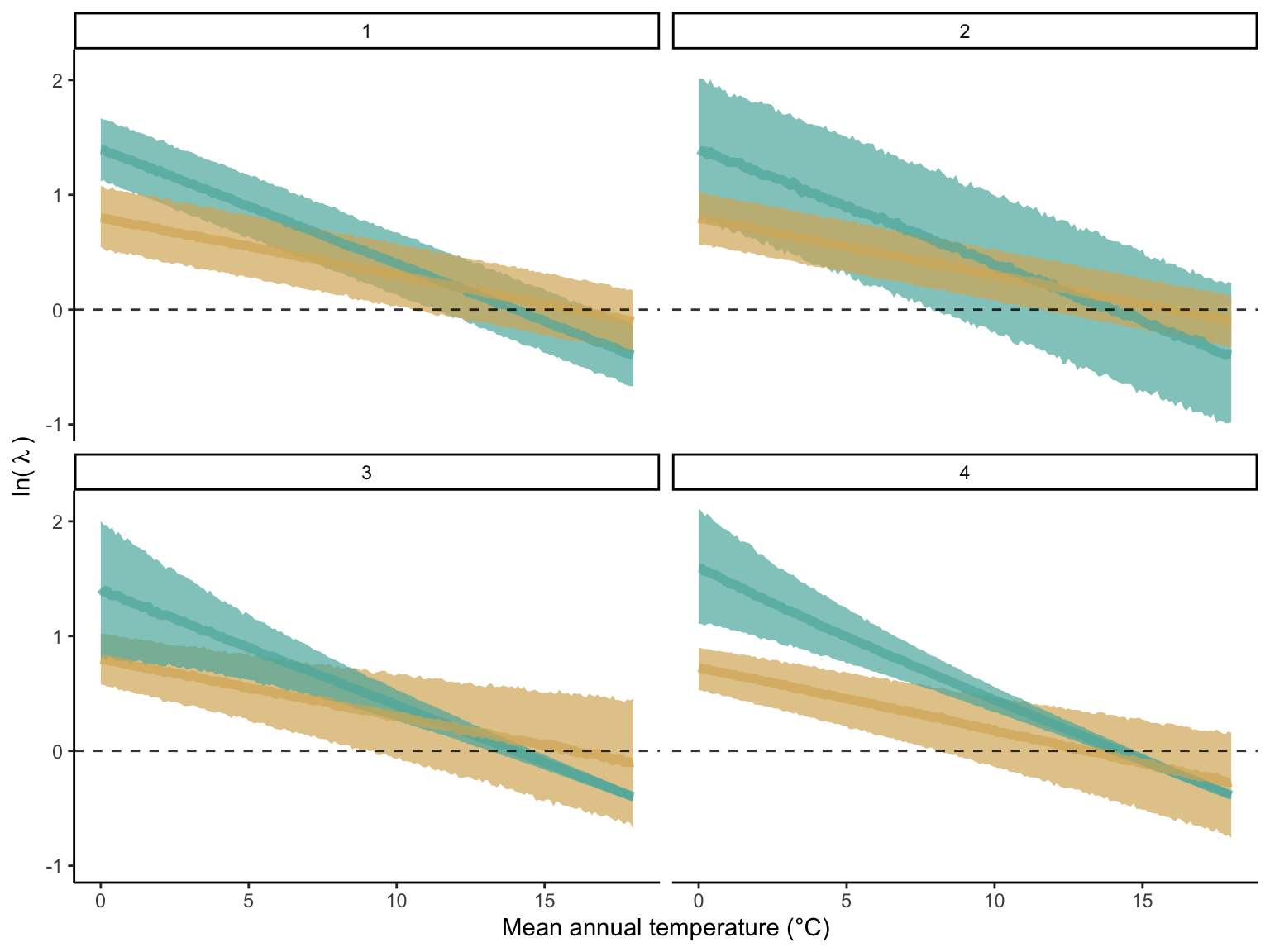
In Figure 21.7, we show some examples of the model’s flexibility. At each panel, two sets of parameter combinations illustrate the different behavior of the model. Each panel illustrates an element of the model attributed to accommodate the data variability. In panel 1, the most straightforward case shows how suitable probability changes linearly with MAT and constant variance. Panel 2 shows two cases with larger and smaller variances derived from the spatiotemporal variability of the conditions and model uncertainty. Panel 3 demonstrates how this variability can change across the range distribution. Finally, panel 4 shows how the asymmetry of the variability can bias the variance towards lower (yellow) or higher (green) values. Note that in panel 4, the illustration does not fully represent the asymmetry in the model, as the tool to create the curves does not allow asymmetric variance. Therefore, while the figure illustrates a shift in the average and variance, we should instead see a shift only in the variance.
Simulations
We computed \(\lambda\) for each species based on the plot-year observations in the dataset, considering both environmentally induced variability and parameter uncertainty. For every observed species-plot-year combination, we incorporated temporal stochasticity in climate conditions by using the mean and standard deviation of mean annual temperature and precipitation calculated from the years between measurements. For instance, in the case of a plot observed twice, we calculated \(\lambda\) for the second observation with climate conditions drawn randomly from a normal distribution with mean and standard deviation defined from climate observations within the year interval. Similarly, temporal stochasticity in competition arises from variation in abundance and composition between measured years. By iteratively performing this calculation, drawing parameter values randomly from the posterior distribution, we introduced demographic uncertainty at the individual level. For each species-plot-year measurement, we replicated the calculation of \(\lambda\) 100 times. By applying this approach across all plots, we naturally incorporate spatial variation in climate and competition conditions and spatial uncertainty in plot-level parameters.
For each species-plot-year-replication combination, we calculated \(\lambda\) under two simulated conditions. The first condition assumed no competition, with heterospecific competition defined at zero and conspecific competition at a minimal proportion (total population size (\(N\)) = 0.1). This condition simulated the population growth rate under the fundamental niche. The second condition simulated the invasion growth rate, representing the population growth rate when the focal species is rare (\(N = 0.1\)) and heterospecific competition set to the observed abundance of the competitive species. This condition simulated the population growth rate under the realized niche. The code for these computations on High-performance computing is available on GitHub: https://github.com/willvieira/forest-IPM/tree/master/simulations/lambda_plot.
After calculating \(\lambda\) for each species-plot-year-replication combination, we used these estimates to fit the linear model describing how \(\lambda\) and its variability change across the mean annual temperature gradient. We fitted the species-specific linear model for the hot and cold ranges using the Hamiltonian Monte Carlo (HMC) algorithm via the Stan software (version 2.30.1 Team et al. 2022) and the cmdstandr R package (version 0.5.3 Gabry, Češnovar, and Johnson 2023). To reduce the sampling time, we used a sample of 5000 plots for each species to fit the model. This sample was necessary only for 6 out of the 31 species. The R and Stan scripts for these computations on High-performance computing are accessible on GitHub: https://github.com/willvieira/forest-IPM/tree/master/simulations/model_lambdaPlot/.
With the fitted models, we leveraged the posterior distribution to estimate the suitable probability of a species for any value of MAT under fundamental or realized niche for the cold and hot ranges. Specifically, we estimated suitable probability under four different MAT conditions encountered by the species: at the border and the center of each cold and hot range. We defined the border of the cold range as the minimum observed MAT for the focal species in the dataset, while the hot range was defined as the maximum observed MAT. The center location is defined as the centroid of MAT for the focal species. Although the center location has the same MAT for the cold and hot ranges, both are retained because the model is fitted separately for the cold and hot ranges. Finally, we estimated suitable probability for each location under no competition (fundamental niche) and heterospecific competition (realized niche) conditions, using the empirical cumulative distribution function over 1000 predictive draws.
Results
Example using Abies balsemea
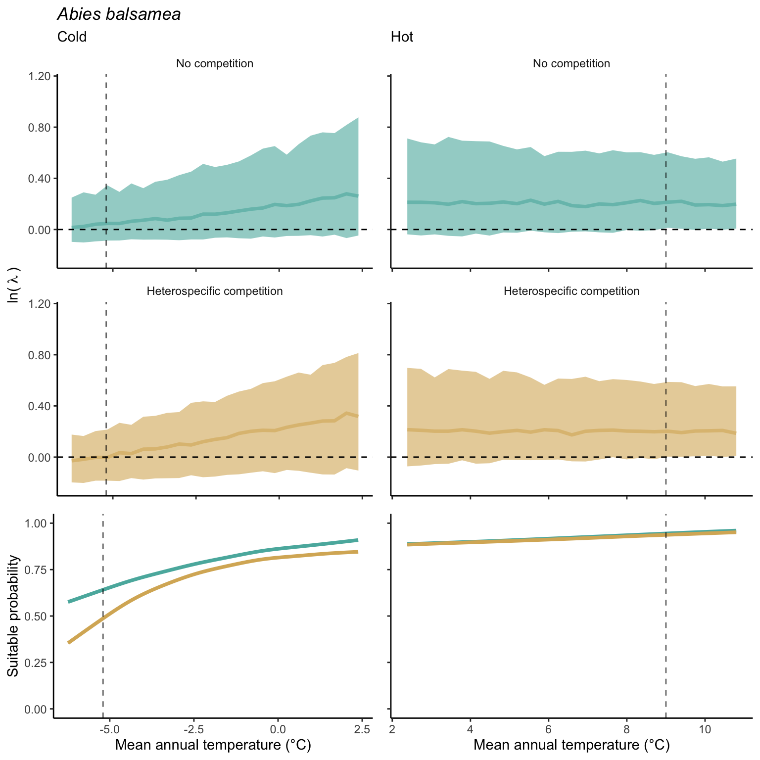
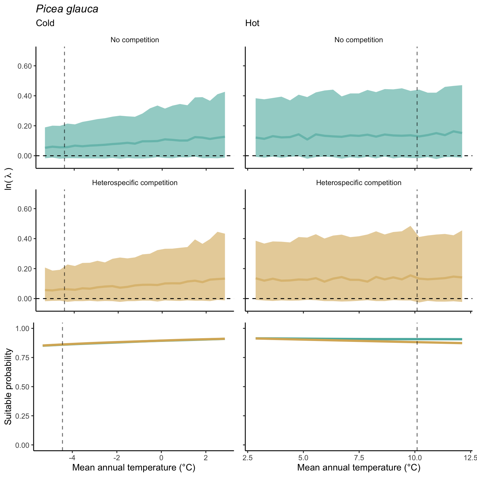
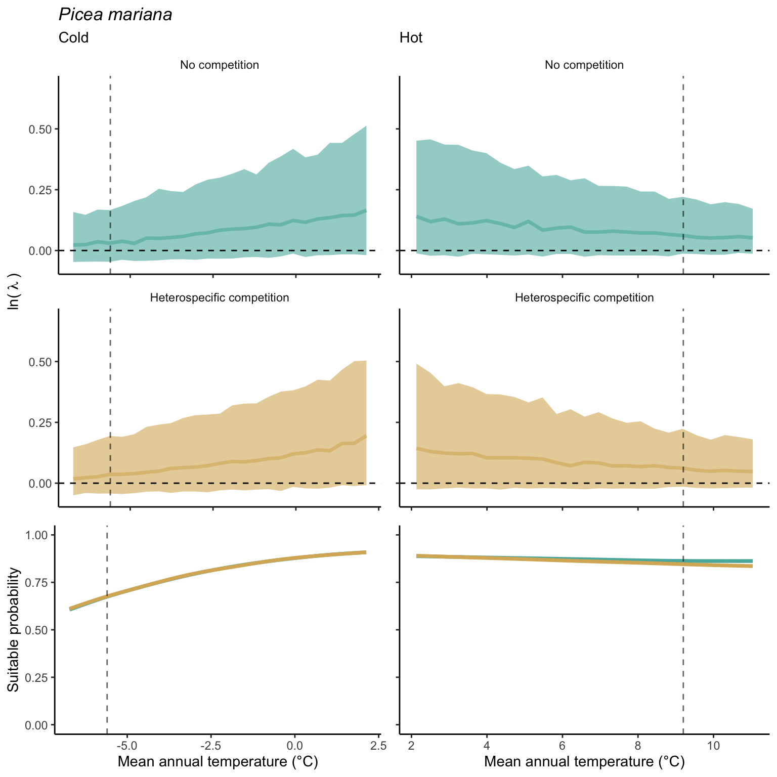
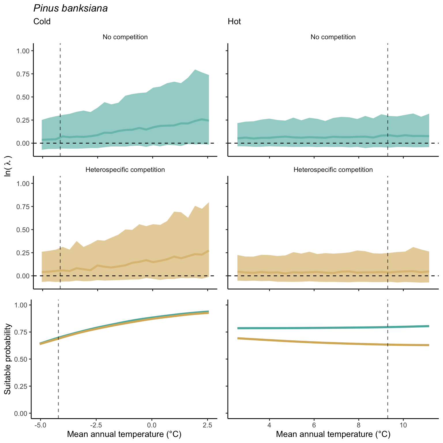
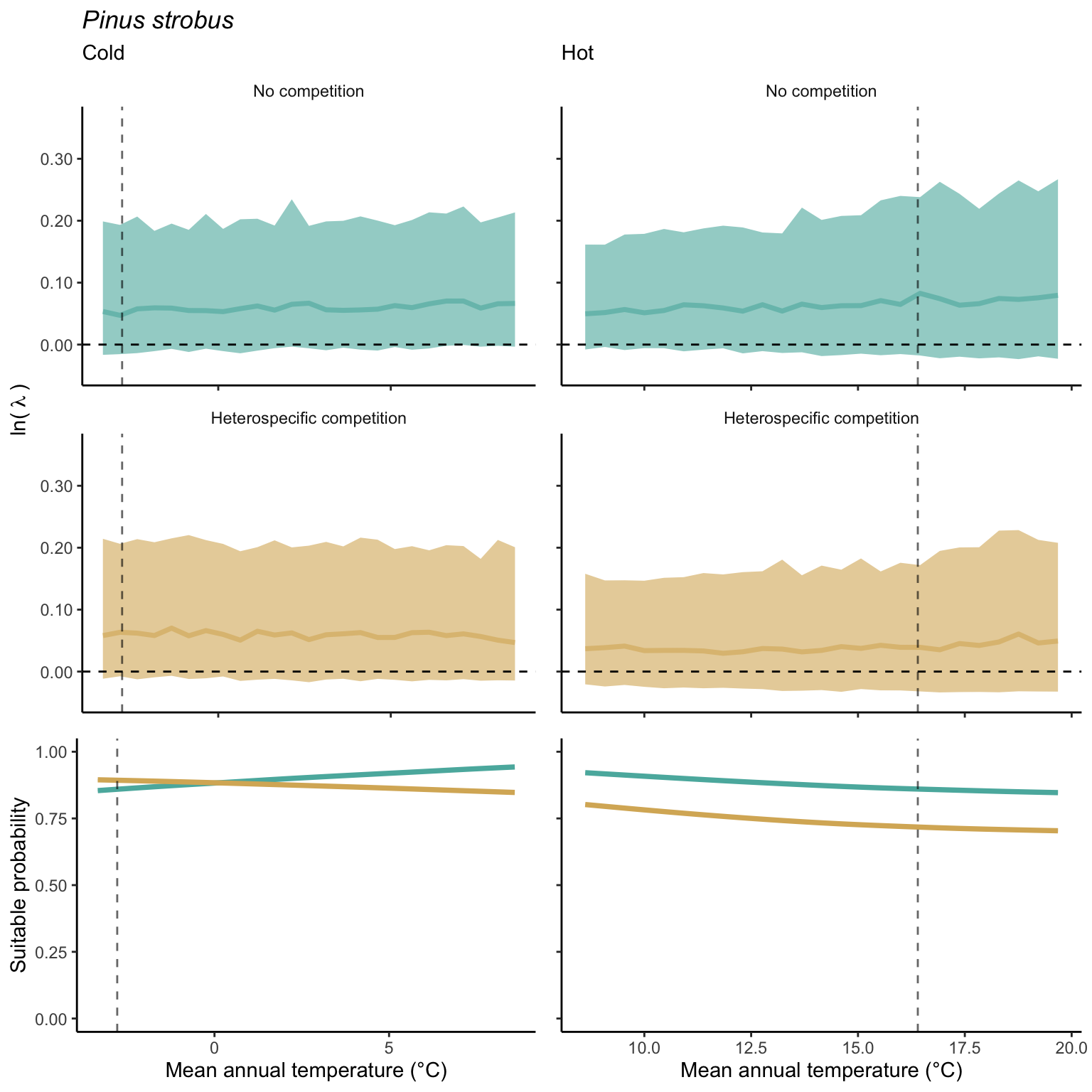
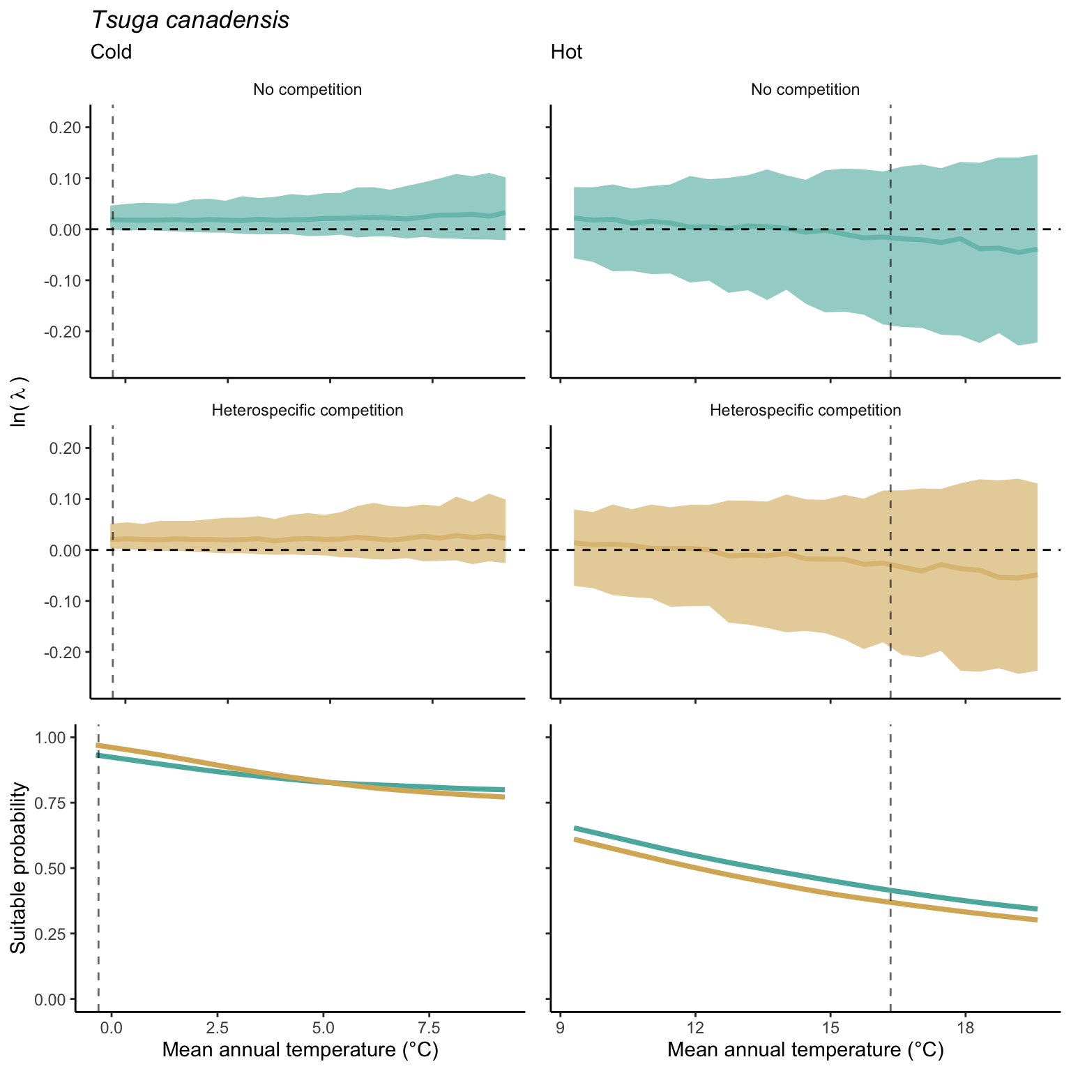
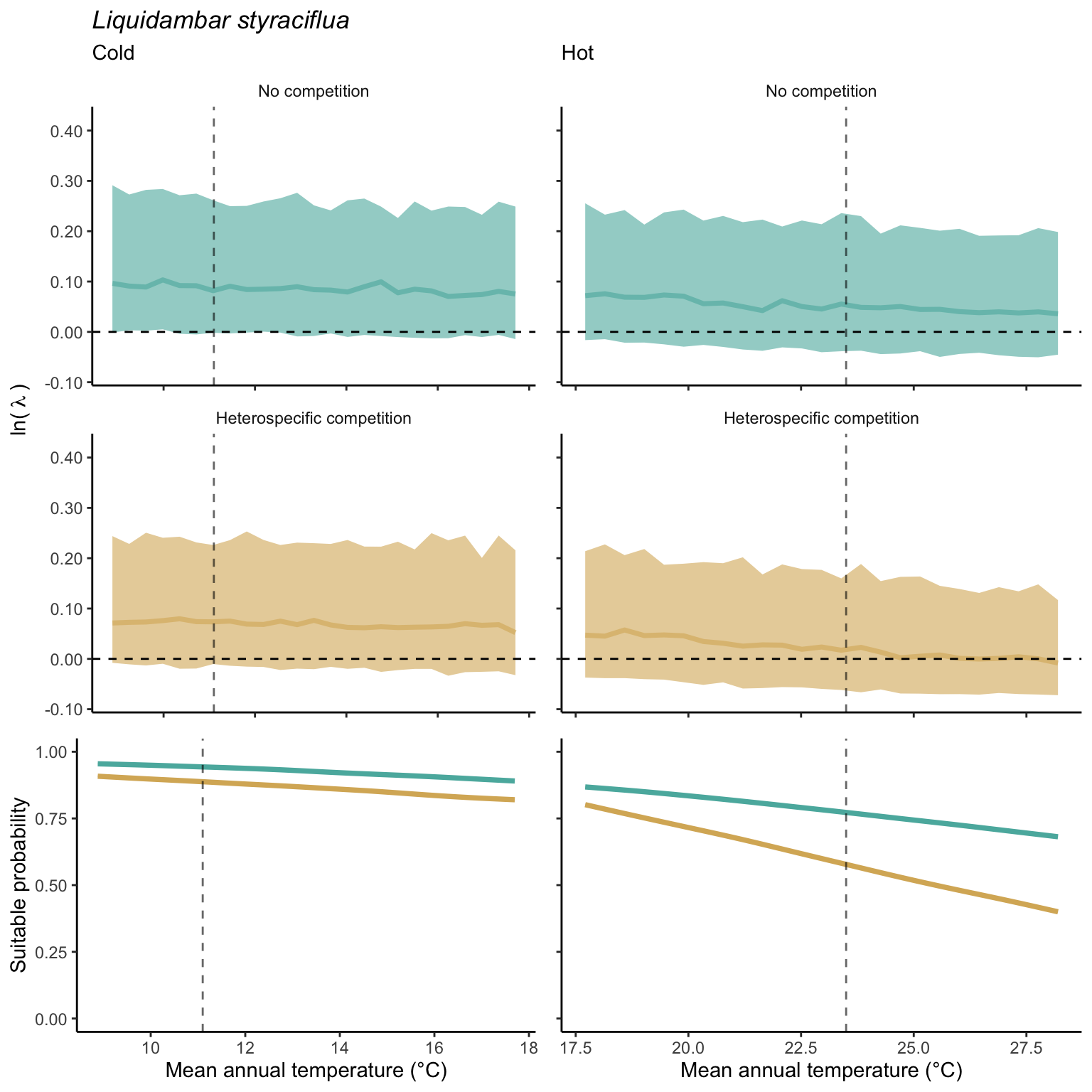
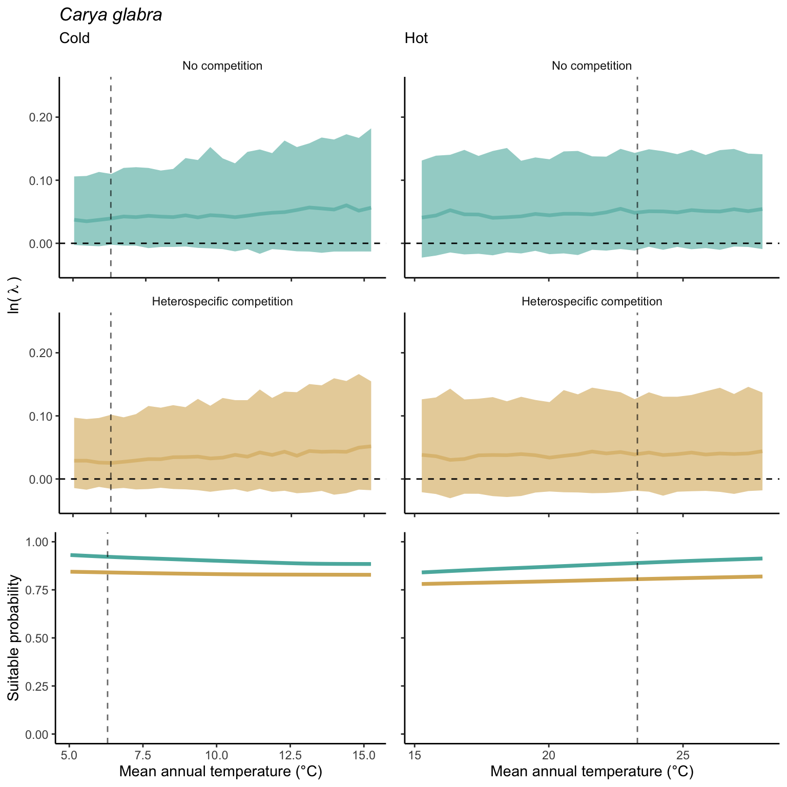
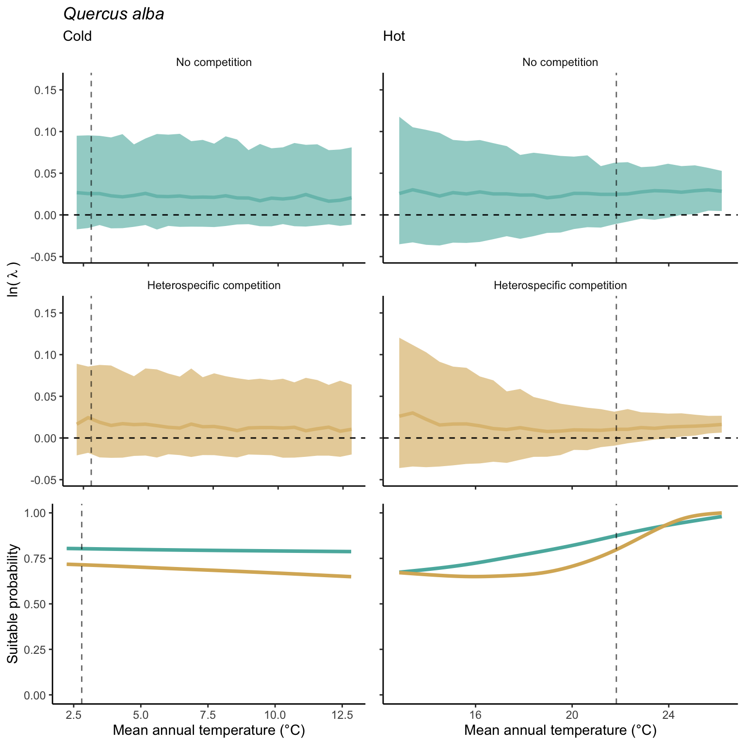
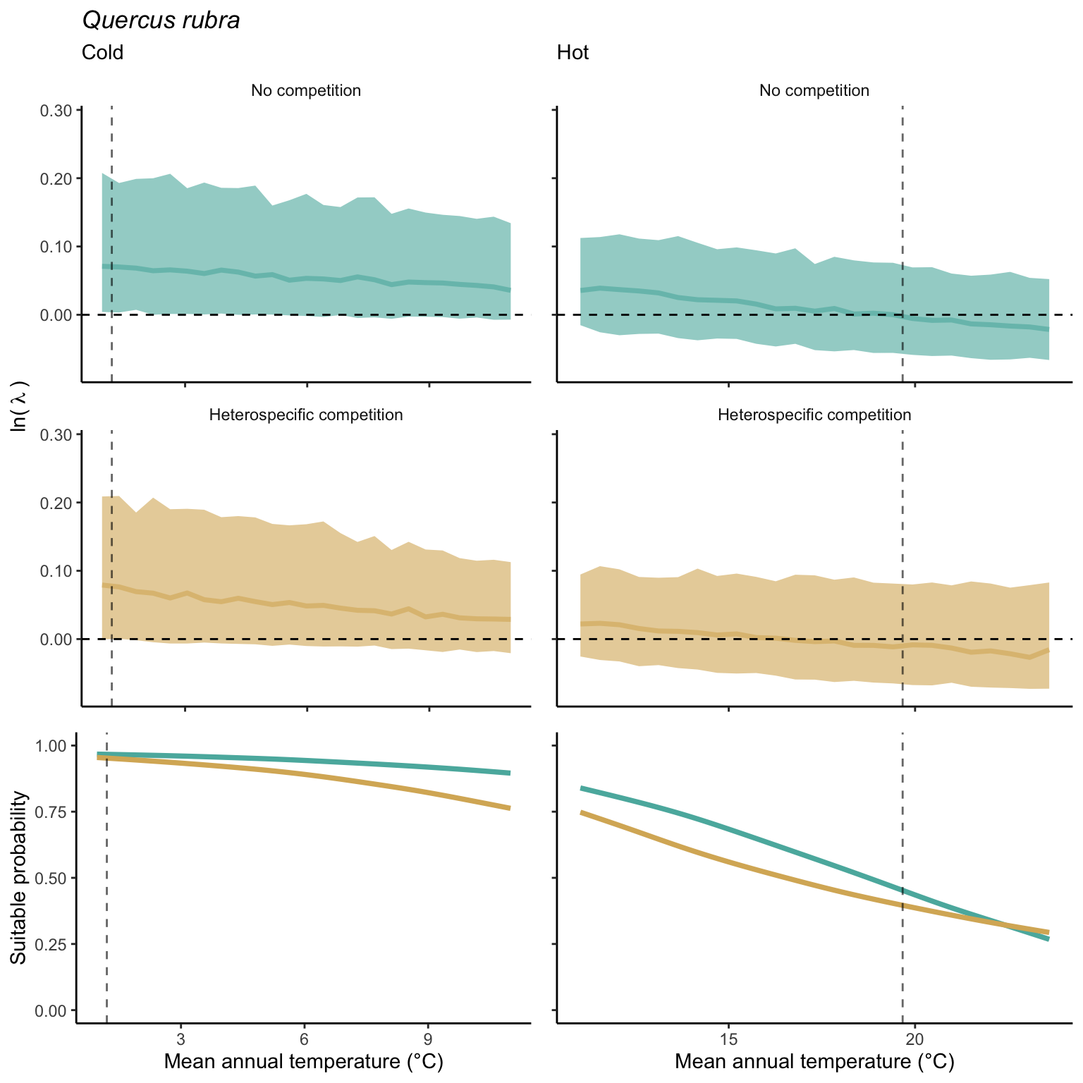
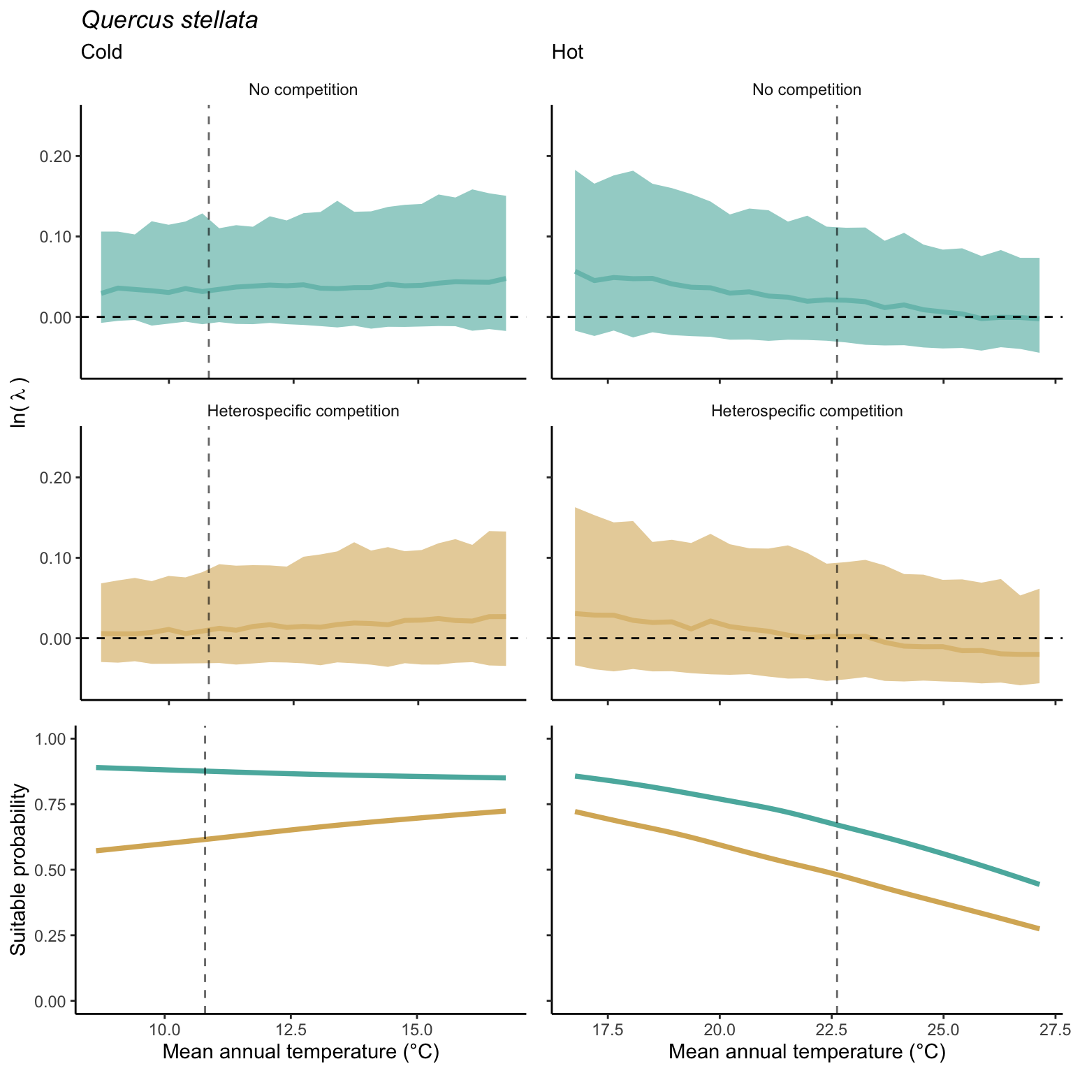
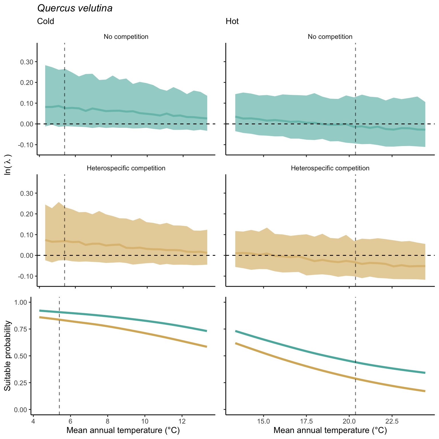
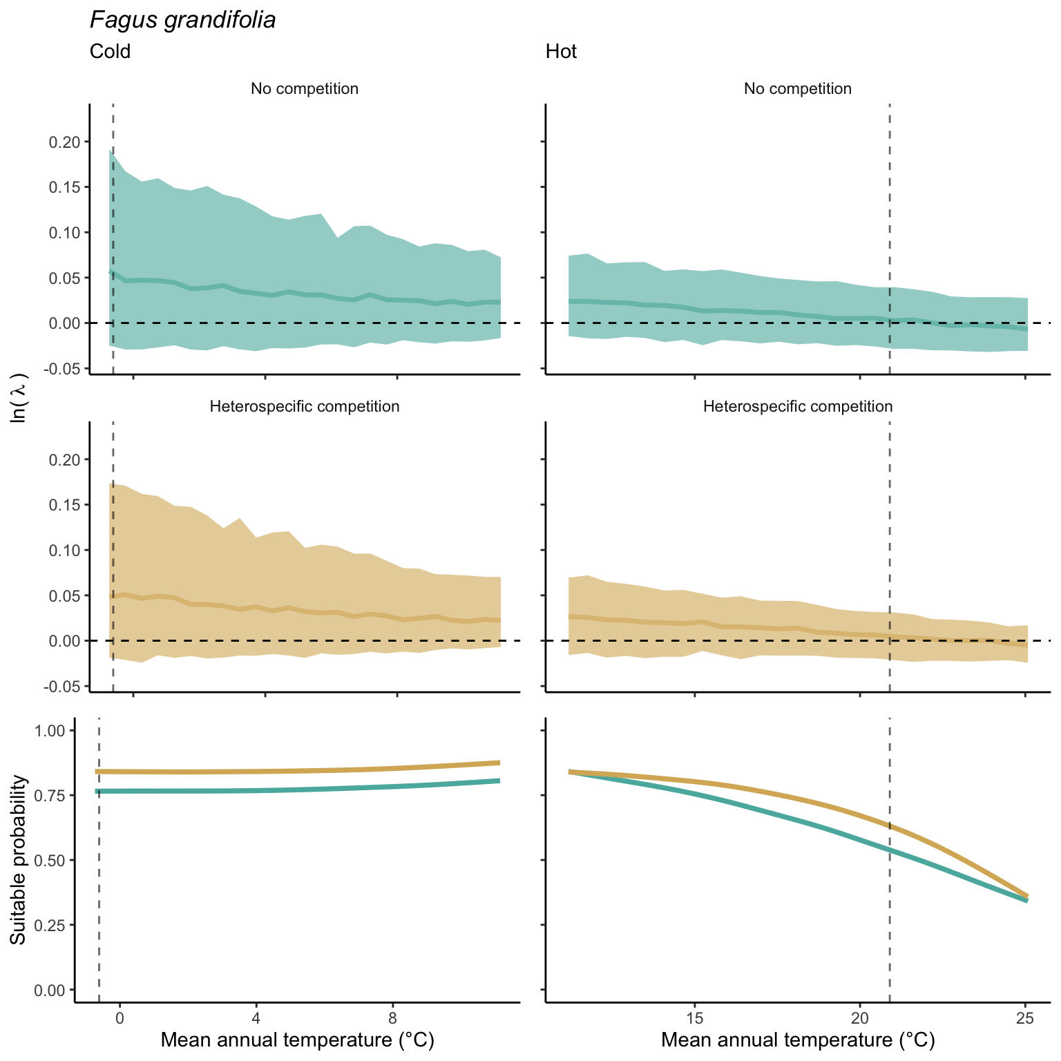
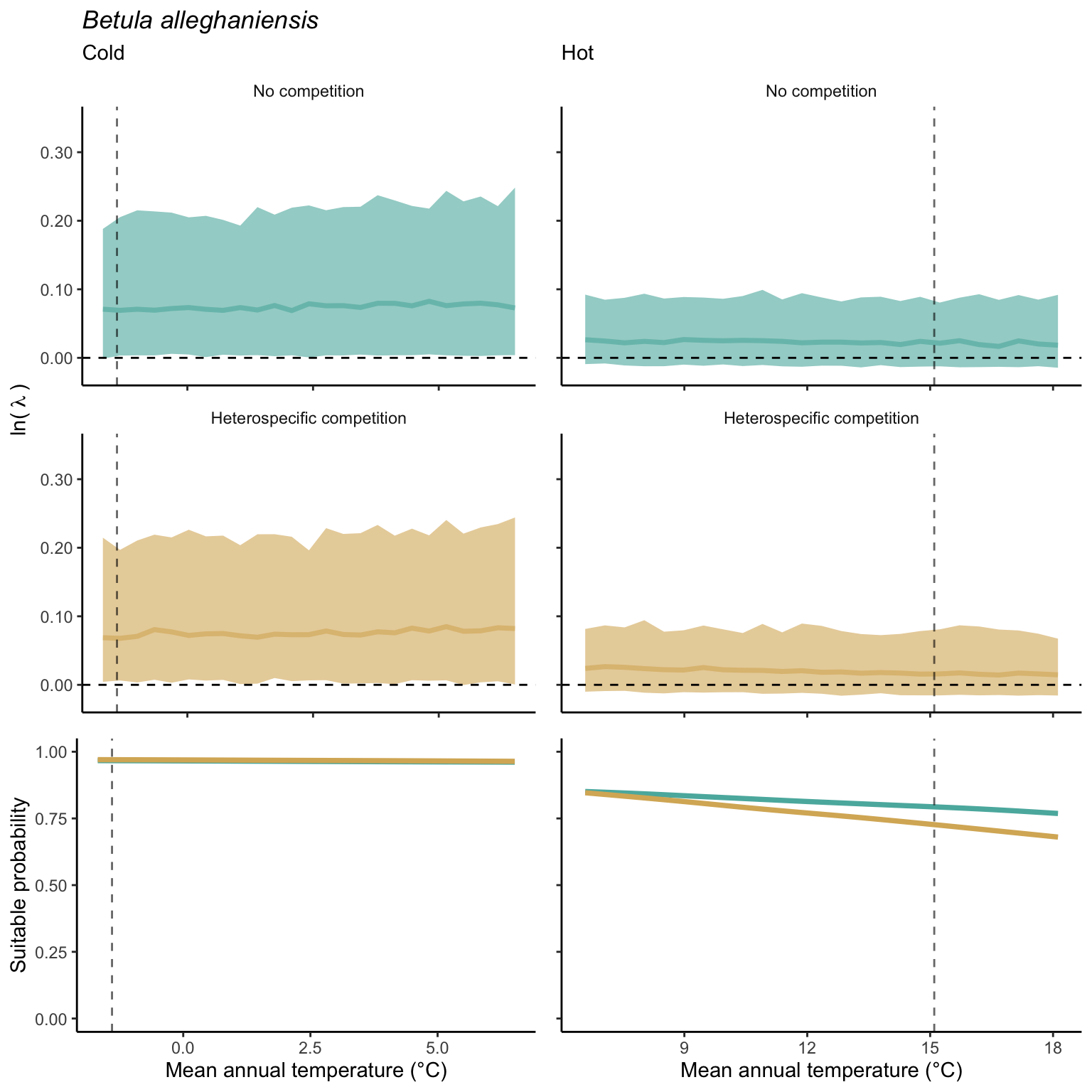
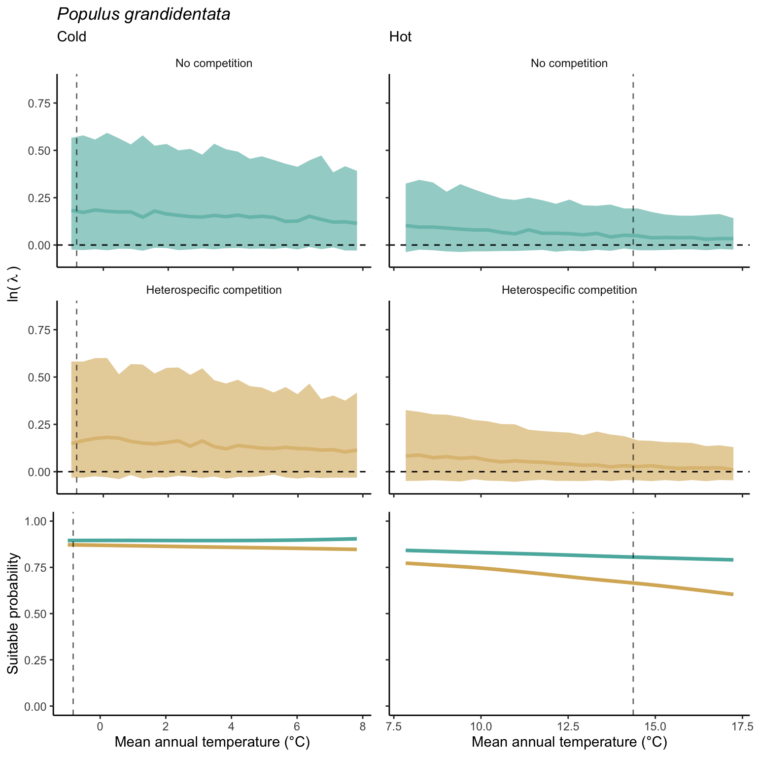
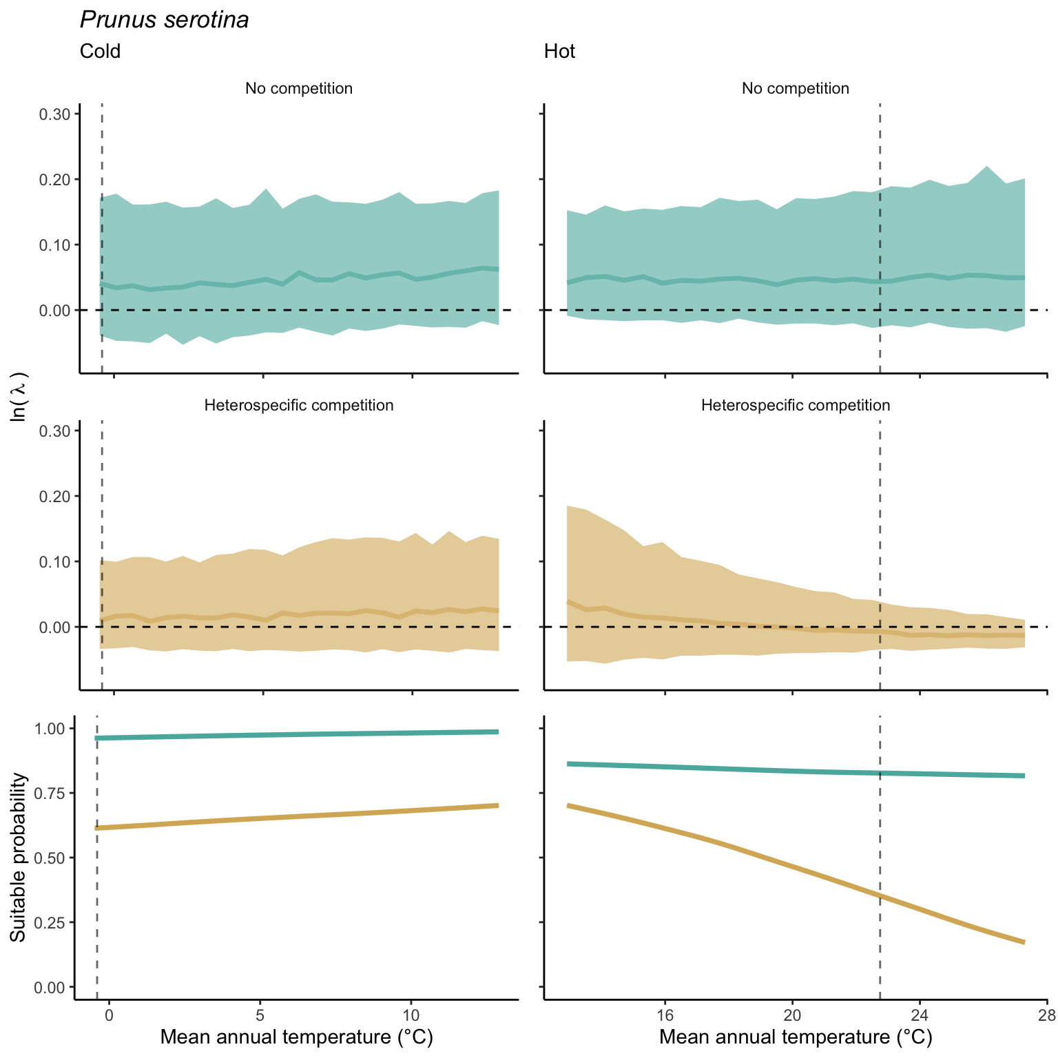
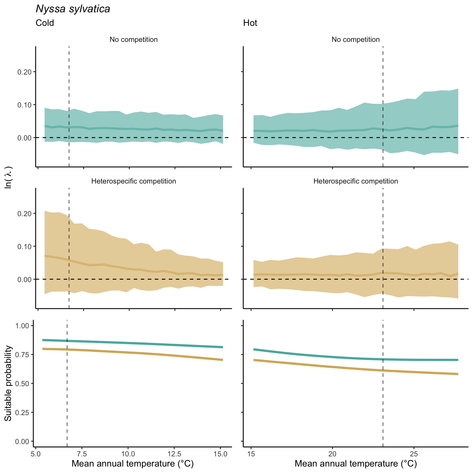
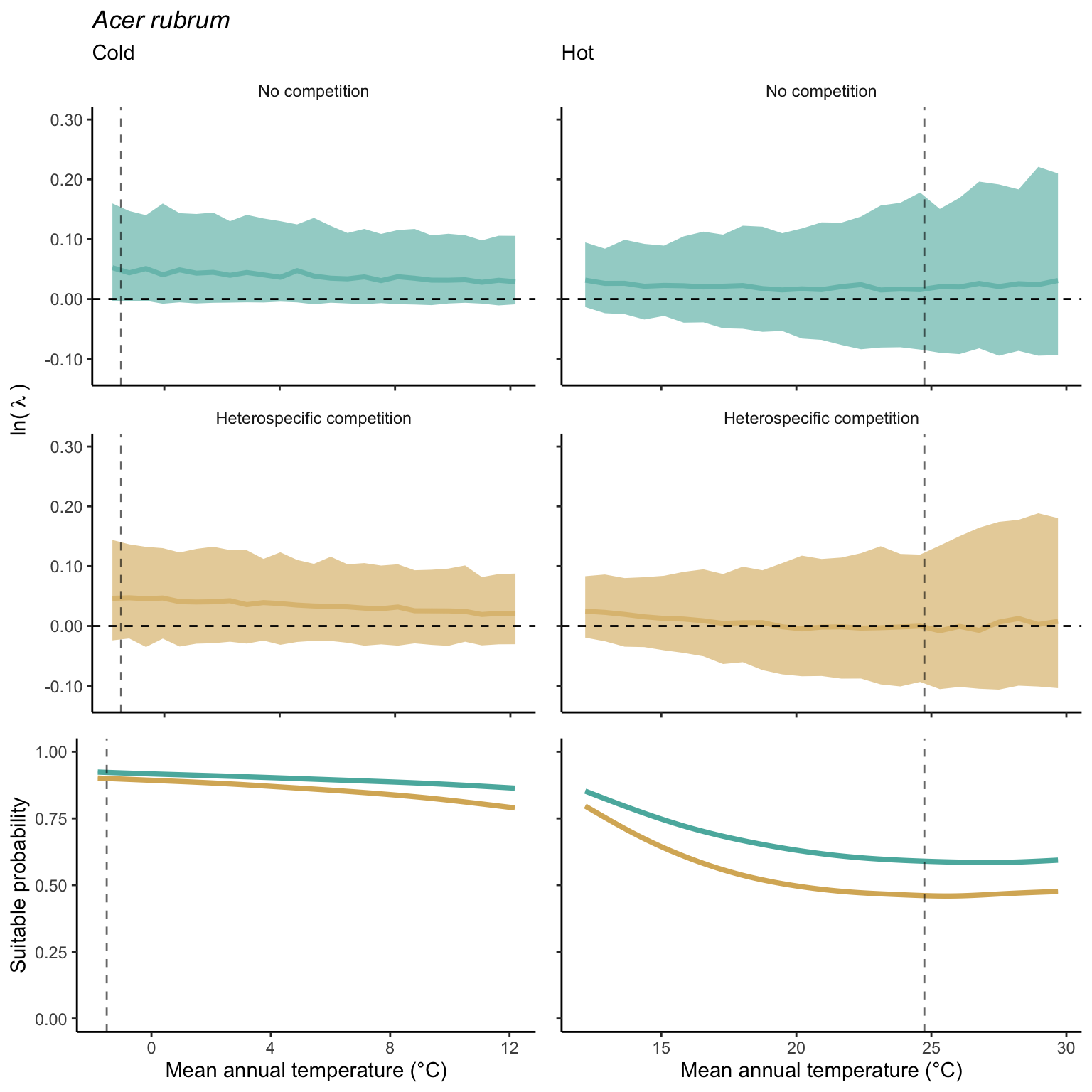
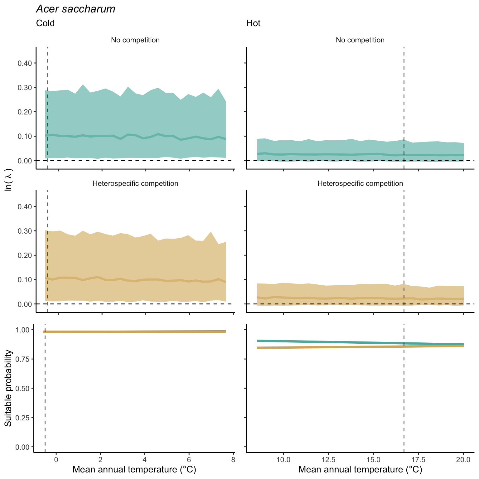
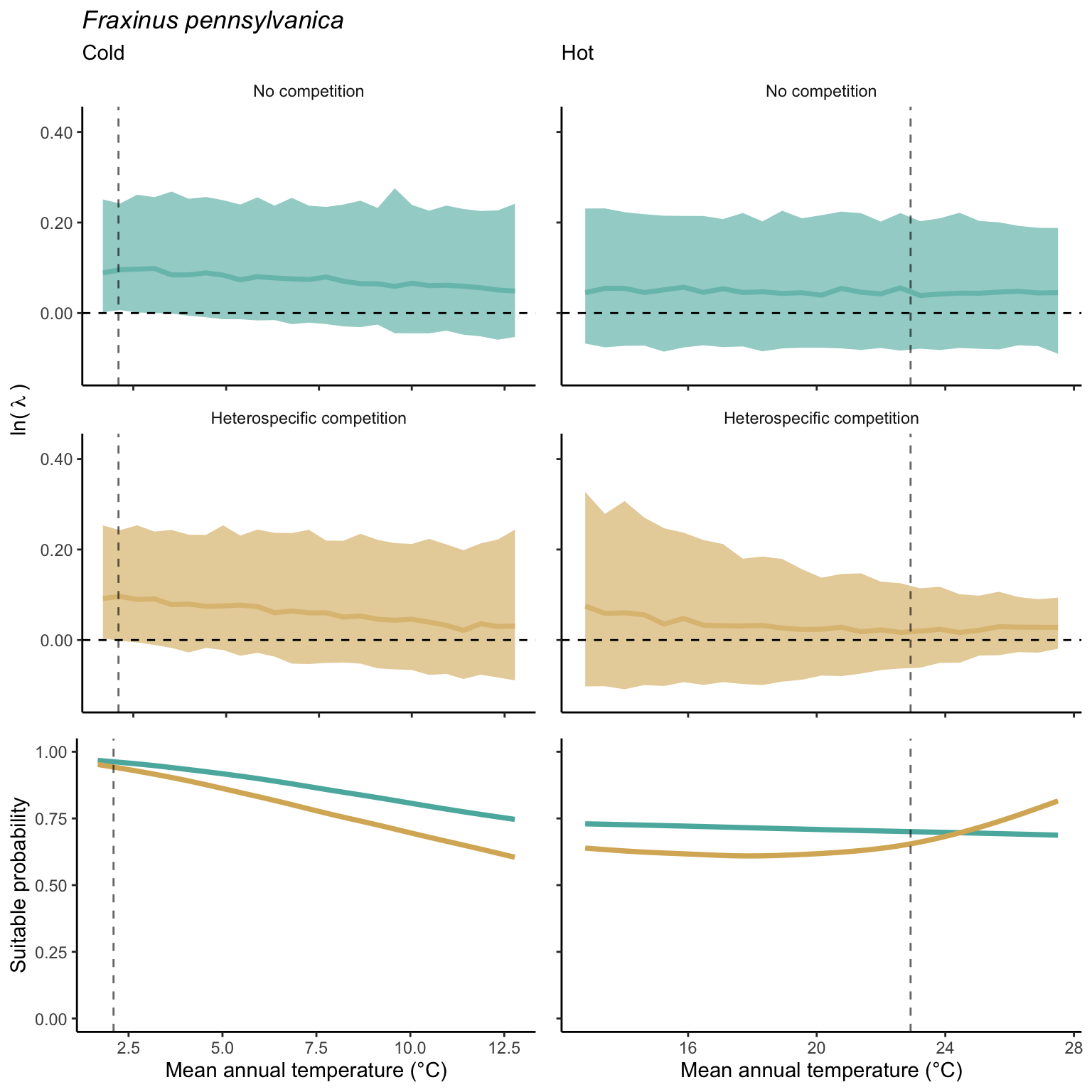
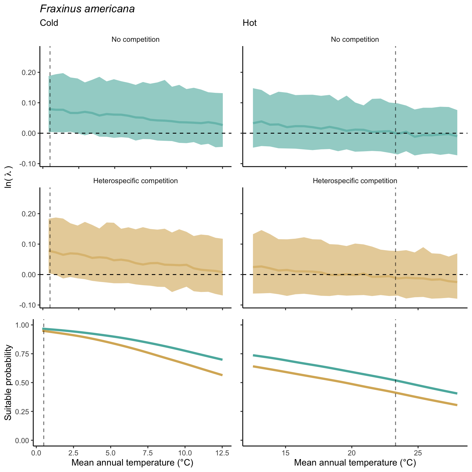
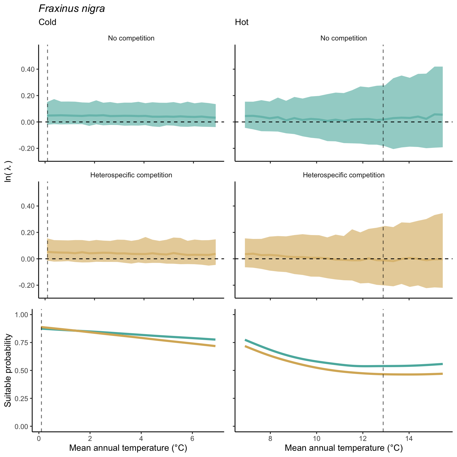
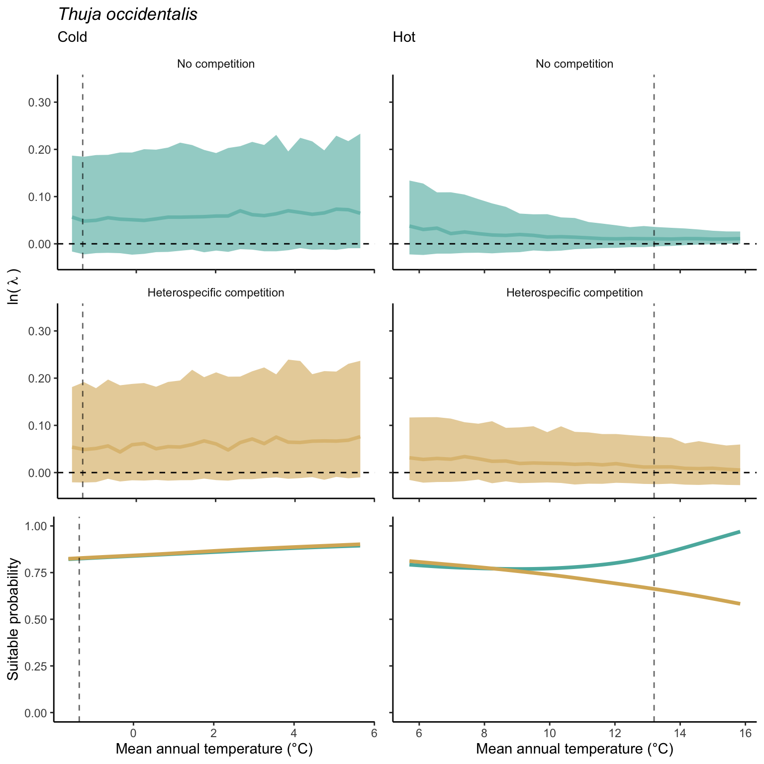
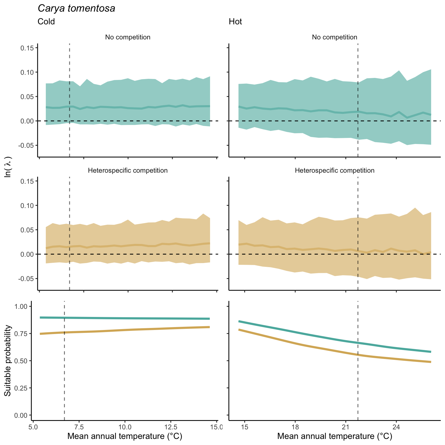
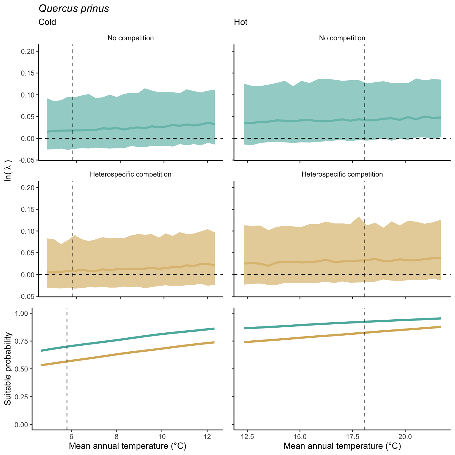
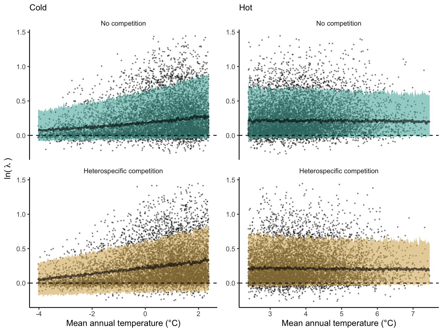
We used a linear model to summarize the evolution of the population growth rate (\(\lambda\)) and its variability across the cold and warm ranges (Equation 21.3). The Figure 21.8 shows the observed \(\lambda\) distribution and the fit of the underlying model on the mean annual temperature gradient for the species Abies balsamea. Each point represents a plot-year-replication encompassing the complete spatio-temporal sources of variability arising from the stochastic environment and parameter uncertainty. The black line represents the average fitted model (how \(\lambda\) changes with MAT), and the shaded area is the 90th quantile of model uncertainty (how the variability of \(\lambda\) changes with MAT). From this uncertainty, we can deduce the suitable probability. In this example, in the cold range, the mean and variance of \(\lambda\) decrease towards the cold boundary. By comparing the model under heterospecific competition with that without competition, we can observe a slight decrease in the average at the cold border but a larger decrease in uncertainty (Figure 21.8 at the bottom left).
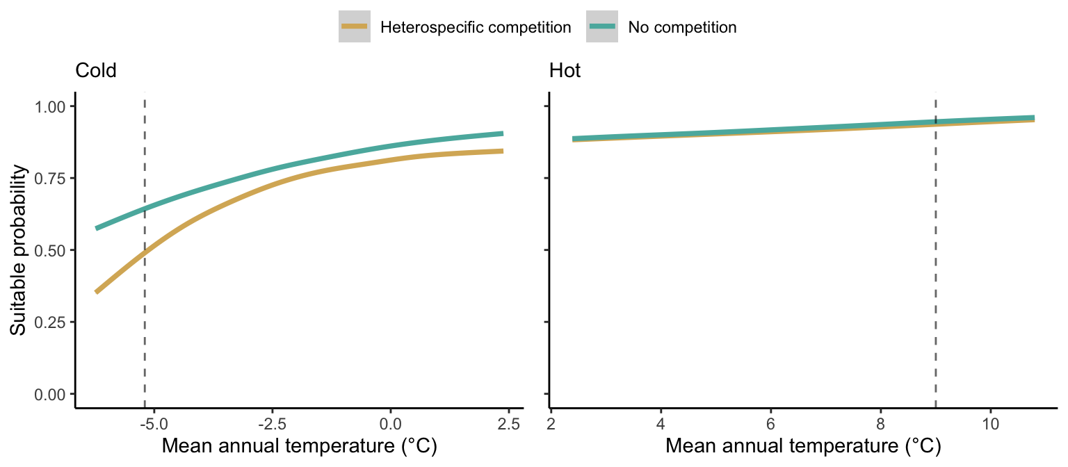
We can estimate the suitable probability using the empirical cumulative distribution approach (Equation 21.2) from the linear model predictions. The Figure 21.9 shows the suitable probability expected over the mean annual temperature of the same species. As expected, the suitable probability was reduced toward the cold border and was lower under heterospecific competition (yellow curve). We can also observe that the decrease in suitable probability toward the border is nonlinear, becoming more substantial for heterospecific competition than for the no-competition condition.
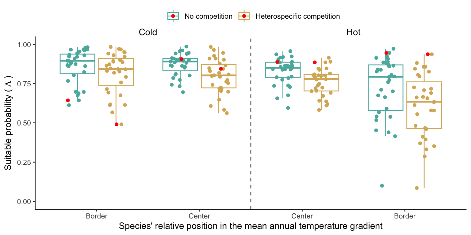
Effect of climate and competition on suitable probability
In the final step, we analyze the effect of competition on the suitable probability at the border and center of the temperature range distribution for all species. The Figure 21.10 compares the suitable probability under no competition to those under heterospecific competition for four locations from the mean annual temperature gradient. Overall, suitable probability was high among the species, with an average of 0.78. Among the four locations, species presented a lower suitable probability at the border of the hot range, with an average of 0.67. Almost all species, in all conditions, are distributed below the identity line (1:1), meaning that heterospecific competition reduces the suitable probability. In the cold range, temperature decrease toward the border had little effect on the suitable probability for both competitive conditions. However, at the hot range, however, we can observe a significant shift in suitable probability from the center to the border. Across the temperature range, there is a monotonic decrease in suitable probability from the cold border toward the hot border.
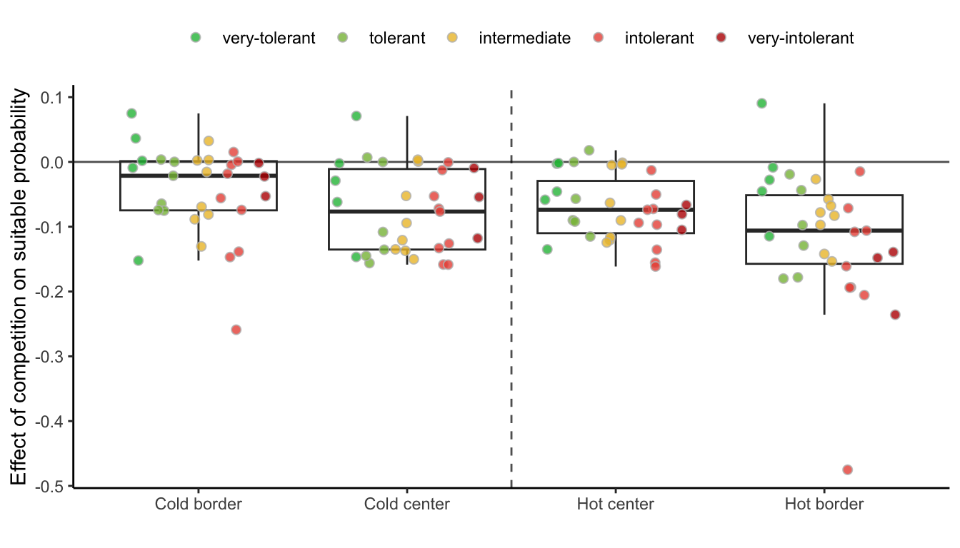
While the negative effect of climate on suitable probability is evident in the above figure, distinguishing the individual effects of competition remains challenging. Hence, in Figure 21.11, we assessed the impact of competition on reducing suitable probability by subtracting the suitable probability under heterospecific competition from the suitable probability with no competition. Even when isolating the effect of climate, the negative impact of heterospecific competition on suitable probability increases toward the border of the hot range.
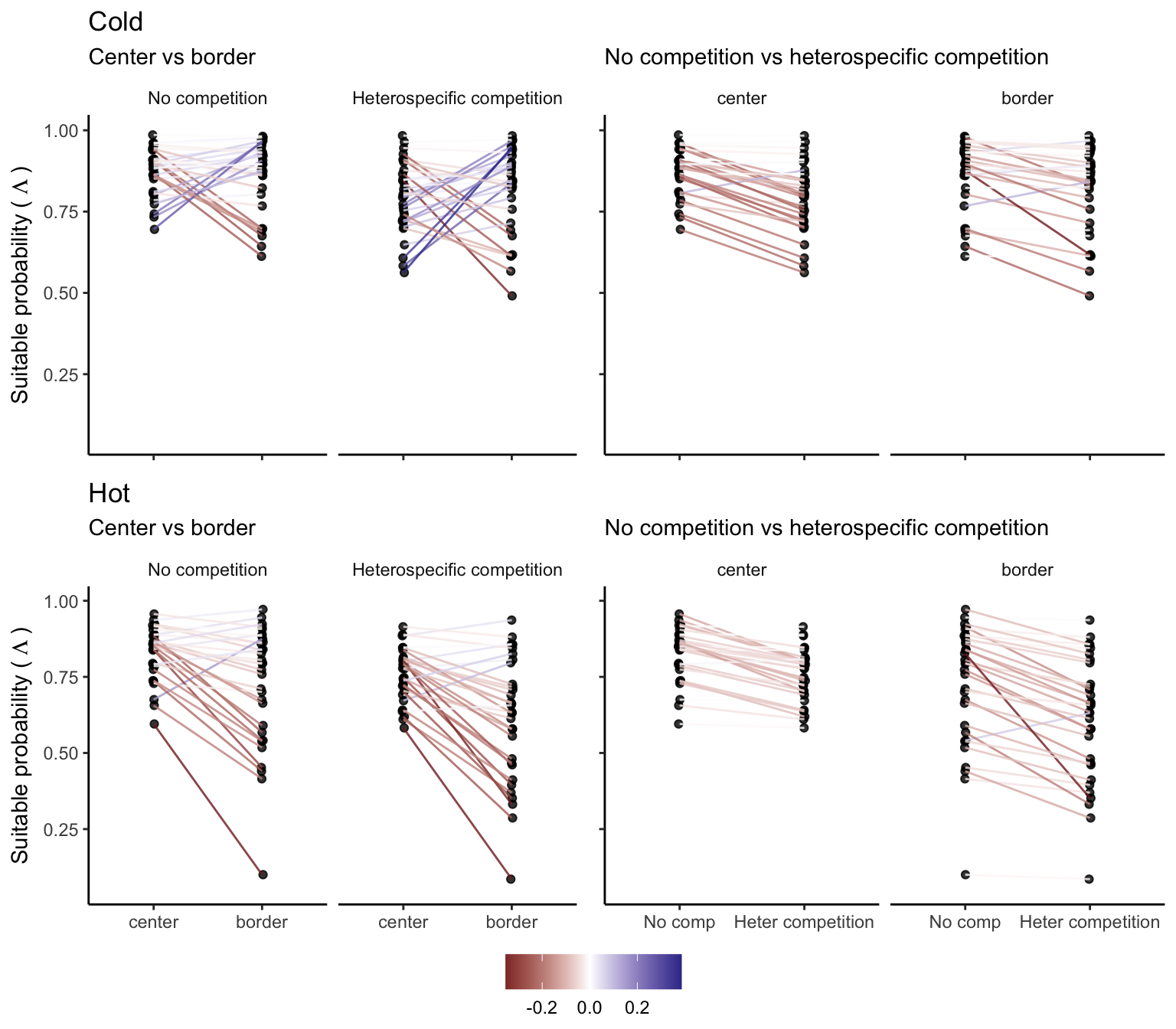
For each species, we estimated the difference in suitable probability between the border and center (for climate) and between heterospecific and non-competition. In Figure 21.12, we compare the suitable probability for each species under the climate or competition conditions, where each line and their respective color determines the amount of change in suitable probability.
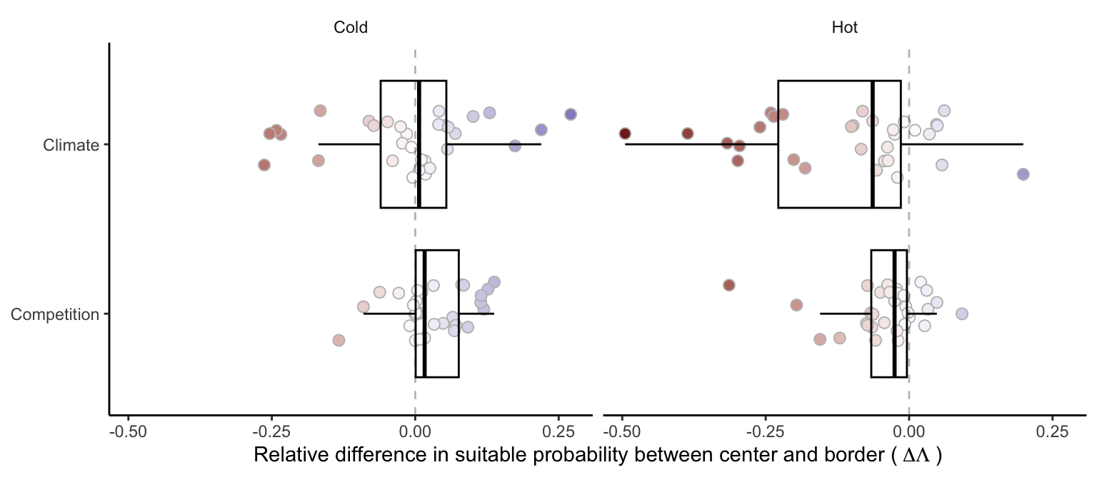
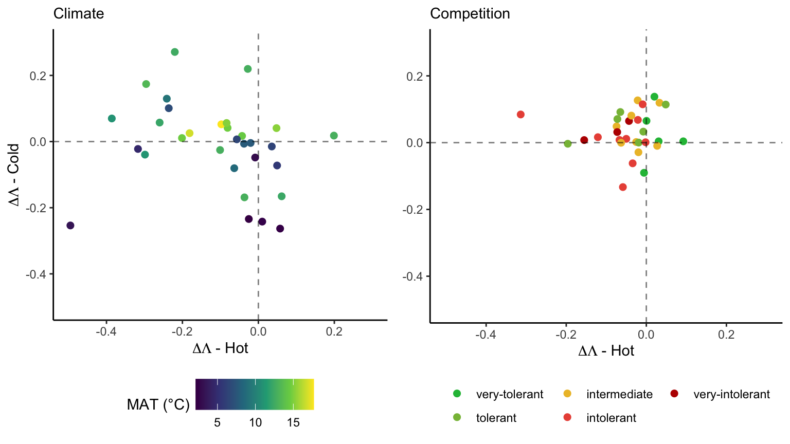
We further estimated the relative effect of climate and competition on changing suitable probability from the center to the border of the species distribution (Figure 21.13). Specifically, we quantified the distinct contributions of temperature and competition to changes in suitable probability. Positive values of the relative difference signify an increase in suitable probability from the center towards the border, negative values indicate a decrease, and zero implies no net change. In the hot range, most species exhibited negative values of the relative difference in suitable probability, indicating a decline in suitability due to higher temperature and intensified competition toward the hot border of the species distribution. At the cold range, most species showed positive values for the competition effect, meaning a reduction in the effect of competition toward the cold border. However, the climate effect at the cold range showed a less clear pattern, with some species experiencing an increase and others a decrease in suitable probability as temperature decreased toward the cold range. Overall, the relative difference in suitable probability from the center toward the border was more influenced by climate rather than competition.
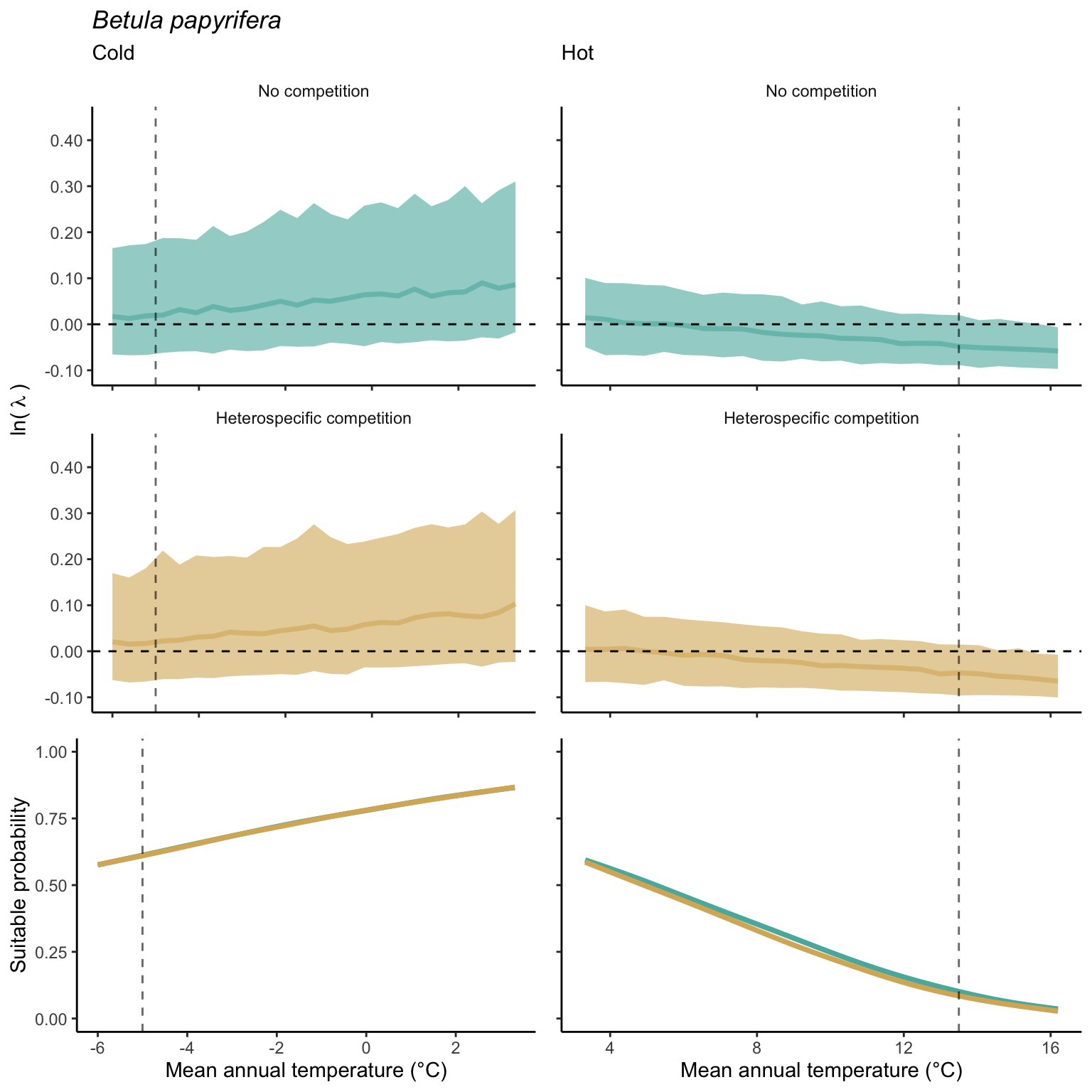
In our investigation of whether suitable probability decreases simultaneously at both borders (indicating a unimodal shape) or exhibits a linear pattern from one border to the other (Figure 21.14), we found distinct patterns under the climate and competition effects. For the climate effect, the majority of species demonstrated a decrease in suitable probability at one border while the other remained unchanged. Additionally, a few species displayed a clear linear pattern of decreasing suitable probability from the cold to the hot border, with only one species (Betula papyrifera) showing a pronounced unimodal shape. Conversely, under the competition effect, most species exhibited a decrease in suitable probability at the hot border and an increase at the cold border, indicating a linear rise in the impact of competition from the cold to the hot border of the distribution.
Suitable probability across the mean annual temperature gradient
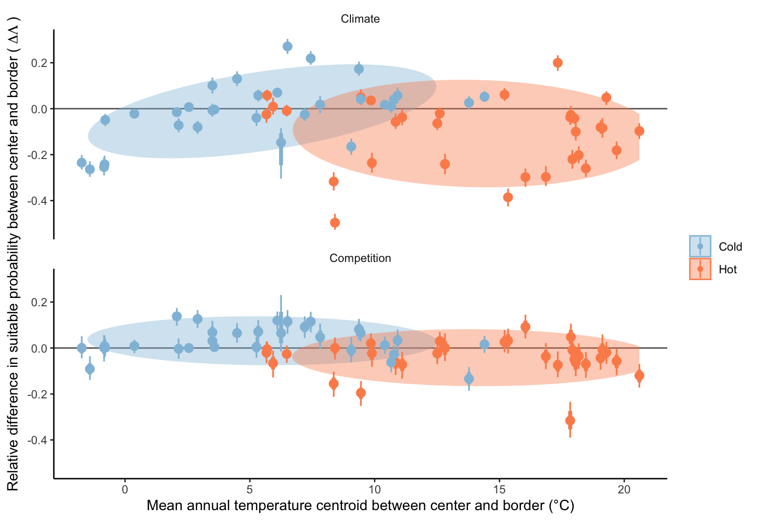
We further investigated the potential dependency of climate and competition effects on the geographical location of the species. Specifically, we hypothesized that the impact of climate might be more pronounced for species distributed in hotter temperatures than those in colder temperatures. In Figure 21.15, we evaluated the difference in suitable probability for climate and competition effects along the mean annual temperature gradient. Notably, the only condition showing a significant trend was the climate effect in the cold range (blue group at the top panel). Not surprisingly, suitable probability decreased as temperature declined toward the cold range, but this pattern was observed only for species located in colder conditions. Conversely, the suitable probability increased when species were situated in hotter conditions as temperature decreased toward the cold range.
Appendices