2  Dataset

This chapter outlines the two data sources and the steps to organize and create a tidy dataset for our analysis. We focus on two open inventory data from eastern North America: the Forest Inventory and Analysis (FIA) dataset in the United States (O’Connell et al. 2007) and the Forest Inventory of Québec (Ministere des Ressources Naturelles 2016). From the FIA dataset, we utilized information collected from 37 states out of the total 50: Alabama, Arkansas, Connecticut, Delaware, Florida, Georgia, Illinois, Indiana, Iowa, Kansas, Kentucky, Louisiana, Maine, Maryland, Massachusetts, Michigan, Minnesota, Mississippi, Missouri, Nebraska, New Hampshire, New Jersey, New York, North Carolina, North Dakota, Ohio, Oklahoma, Pennsylvania, Rhode Island, South Carolina, South Dakota, Tennessee, Texas, Vermont, Virginia, West Virginia, and Wisconsin.

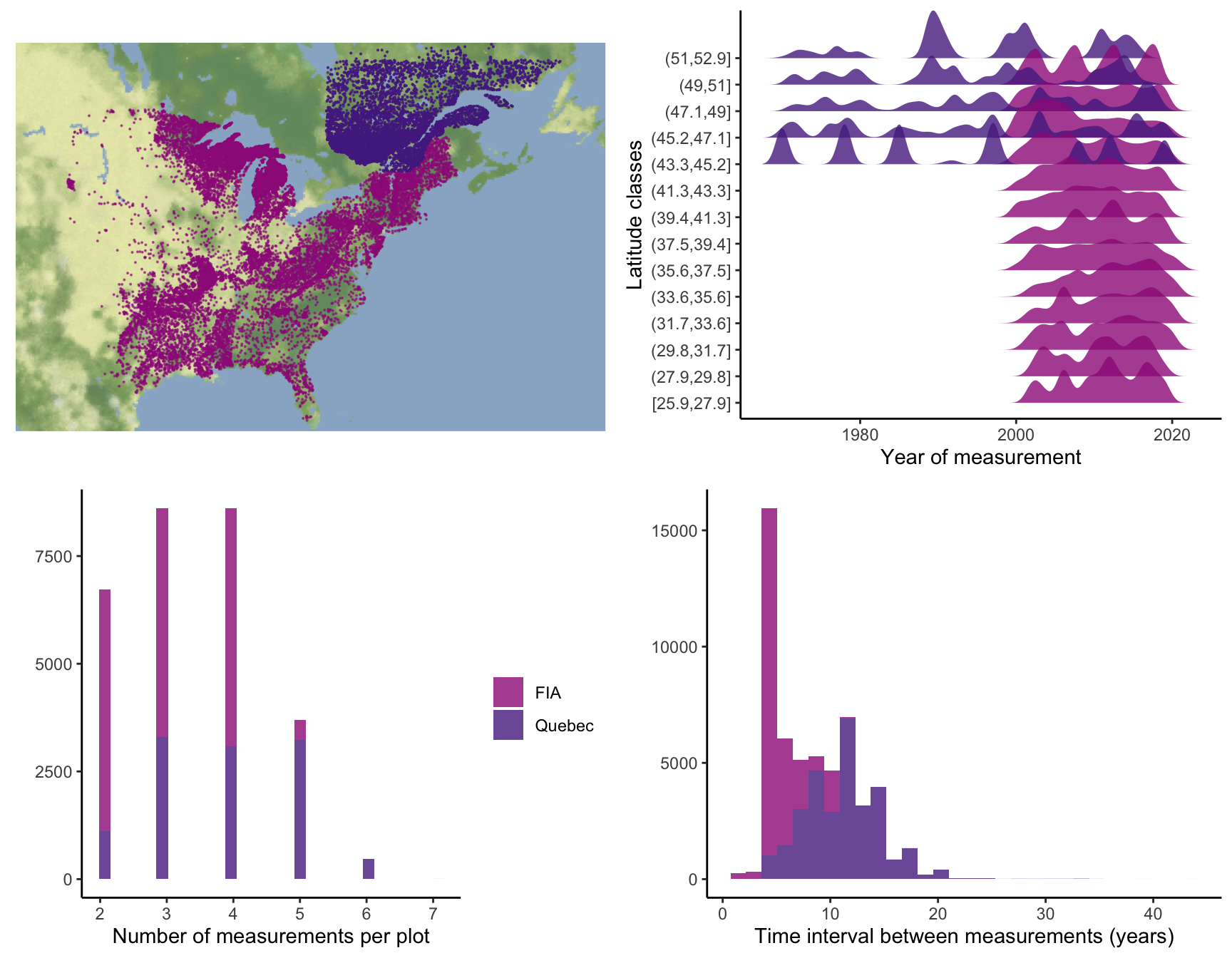
At the plot level, we retained plots sampled at least twice, excluding those that had undergone harvesting to focus solely on natural dynamics. Specifically, we selected surveys conducted for the FIA dataset using the modern standardized methodology implemented since 1999. After applying these filters, our final dataset encompassed nearly 26,000 plots spanning a latitude range from 26° to 53° (Figure 2.1). Each plot within the dataset was measured between 1970 and 2021, with observation frequencies ranging from 2 to 7 times and an average of 3 measurements per plot. The time intervals between measurements varied from 1 to 40 years, with a median interval of 7 years (Figure 2.1).

Figure 2.1: Spatial (top left) and temporal (top right) coverage of the dataset incorporating data from the USA and Quebec. The top right panel shows the distribution of observations per class of latitude for the 31 species used in this study.

These datasets provide individual-level information on the diameter at breast height (dbh) and the status (dead or alive) of more than 200 species. From this pool, we selected the 31 most abundant species (Table 2.1). This selection comprises 9 conifer species and 21 hardwood species. We ensured an even distribution of species across the continuous shade tolerance trait, with 3 species classified as very intolerant, 9 as intolerant, 8 as intermediate, 8 as tolerant, and 5 as very tolerant (Burns, Honkala, et al. 1990). While our analysis focuses on these 31 selected species, we retained the data for the remaining species for potential future exploration and analysis. We initially included the Ostrya virginiana species in our analysis; however, we encountered substantial challenges with several growth, survival, and recruitment parameters, with substantial confidence intervals. As a result, we decided to remove this species from our analysis, even though the fit files are still accessible for potential future investigations.

Table 2.1: List of species and their frequency across the dataset.

Species	Species ID	Number of plots	Number of individual	Number of observation
Acer rubrum	28728ACERUB	13149	96739	235408
Abies balsamea	18032ABIBAL	11932	247737	521565
Betula papyrifera	19489BETPAP	9508	78049	203500
Picea mariana	183302PICMAR	7869	186491	454246
Acer saccharum	28731ACESAC	7403	71961	184641
Picea glauca	183295PICGLA	5889	27641	65626
Populus tremuloides	195773POPTRE	5876	56010	127115
Betula alleghaniensis	19481BETALL	5624	28872	73116
Quercus rubra	19408QUERUB	4549	18272	46341
Quercus alba	19290QUEALB	4200	20376	51466
Fagus grandifolia	19462FAGGRA	3819	21784	51764
Prunus serotina	24764PRUSER	3730	12178	26464
Thuja occidentalis	505490THUOCC	3230	51312	125811
Pinus strobus	183385PINSTR	3165	15638	38470
Fraxinus americana	32931FRAAME	2885	8942	21501
Quercus velutina	19447QUEVEL	2722	10068	23298
Tsuga canadensis	183397TSUCAN	2604	17914	45198
Nyssa sylvatica	27821NYSSYL	2436	6275	15785
Quercus stellata	19422QUESTE	2279	14707	32102
Picea rubens	18034PICRUB	2190	16580	41674
Liquidambar styraciflua	19027LIQSTY	2154	11655	29671
Fraxinus pennsylvanica	32929FRAPEN	2149	9048	20588
Tilia americana	21536TILAME	2059	8415	21412
Pinus banksiana	183319PINBAN	2057	34122	75372
Populus grandidentata	22463POPGRA	2015	13759	29358
Fraxinus nigra	32945FRANIG	1951	12633	31156
Liriodendron tulipifera	18086LIRTUL	1912	8580	21071
Carya tomentosa	NACARALB	1636	3897	10590
Carya glabra	19231CARGLA	1622	4002	9916
Quercus prinus	NAQUEPRI	1590	11000	27554
Juniperus virginiana	18048JUNVIR	1571	9474	21400

Covariates

Competition index

To assess competition effects, we calculated the basal area (BA) of living individuals for each species-plot-year combination based on the dbh of each \(i\). We first calculated individual BA in \(m^2\) as follows:

\[ BA^{ind}_i = \pi * (\frac{dbh_i}{2 * 1000})^2 \]

where the dbh is measured in millimeters. For a given plot \(j\), the total plot basal area in square meters per hectare (\(m^2 ha^{-1}\)) is defined as:

\[ BA^{plot}_j = \sum_i^{n_j}{BA^{ind}_i} \times \frac{10000}{plot~area_j} \]

To compute the basal area of larger individuals (BAL), we summed the total basal area of individuals whose dbh exceeded that of the focal individual \(i\) (\(n_j > BA_i\)):

\[ BAL^{plot}_{ij} = \sum_i^{n_j > BA_i}{BA^{ind}_i} \times \frac{10000}{plot~area_j} \]

Note that BAL is now specific to the plot (\(j\)) and the individual (\(i\)).

Climate

We obtained the 19 bioclimatic variables with a 10 \(km^2\) (300 arcsec) resolution grid, covering the period from 1970 to 2018. These climate variables were modeled using the ANUSPLIN interpolation method (McKenney et al. 2011). We used the plot’s longitude and latitude coordinates to extract the mean annual temperature (MAT) and mean annual precipitation (MAP). To incorporate the climate covariates in the dataset, we used each plot’s latitude and longitude coordinates to extract the mean annual temperature (MAT) and mean annual precipitation (MAP). In cases where plots did not fall within a valid pixel of the climate variable grid, we interpolated the climate condition using the eight neighboring cells. Due to the transitional nature of the dataset, we considered both the average and standard deviation of MAT and MAP over the years within each time interval. This approach allows us to account for climate’s averaged and temporal variability effects on tree demography. Finally, we normalized MAT and MAP within the 0 and 1 range, facilitating comparisons of optimal climate conditions and climate breadth among species.

R objects

All the scripts for dataset preparation are available at https://github.com/willvieira/TreesDemography within the R folder. These scripts detail the complete process of downloading, cleaning, and merging the data, resulting in the final datasets used in our study. Metadata associated with each script is described in Table Table 2.2.

• treeData.RDS: This file contains the complete dataset in a tidy format, with one observation per row.

From the treeData.RDS dataset, we derived four additional datasets, each representing the transition between time \(t\) and time $t + t`:

• growth_dt.RDS: Contains growth rate information between time \(t\) and \(t + \Delta t\).
• status_dt.RDS: Contains individuals’ status (alive or dead) at both time \(t\) and time \(t + \Delta t\).
• fec_dt.RDS: Contains ingrowth rate (number of individuals entering the population at 127 mm) between time \(t\) and \(t + \Delta t\).
• sizeIngrowth_dt.RDS: Contains the size distribution of all individuals that entered the population for each remeasurement.

You can access all the data objects mentioned in the ownCloud folder via this link: doc.ielab.usherbrooke.ca/s/83YSAiLAGeLm682. In addition to the data objects, this folder contains three extra files:

• climate_scaleRange.RDS contains the maximum and minimum values required to scale the climate covariates.
• db_metadata.csv contains the csv description used in the table below.
• species_id.csv contains species descriptions and additional traits used in the analysis.

Table 2.2: Description of metadata for each variable linked to its corresponding dataset object (R object). Note that replicated variables shared among the R objects have been excluded. Consequently, there is no detailed description for the sizeIngrowth_dt dataset.

R object	Variable	Description
treeData	plot_id	plot ID
treeData	longitude	longitude crs(4326)
treeData	latitude	latitude crs(4326)
treeData	plot_size	size of plot in m2
treeData	BA_plot	total plot basal area of alive individuals (m2/ha)
treeData	BA_comp	plot basal area of larger individuals (m2/ha)
treeData	relativeBA_comp	deprecated
treeData	s_star	the height in which the canopy closes (meters)
treeData	db_origin	if FIA or Quebec
treeData	bio_01_mean	mean of mean annual temperature for the years within the time interval
treeData	bio_12_mean	standard deviation of mean annual temperature for the years within the time interval
treeData	bio_01_sd	same as bi_01_mean, but for mean annual precipitation climate variable
treeData	bio_12_sd	same as bio_01_sd, but for mean annual precipitation climate variable
treeData	climate_cellID	the climate cell ID in which the plot climate variables were extracted (similar between MAT and MAP
treeData	tree_id	the unique ID for an individuala tree
treeData	species_id	species unique ID following the`species_id.csv` metadata file
treeData	status	0 = dead; 1 = alive
treeData	year_measured	year of field measurement
treeData	dbh	diameter at breast height of the individual tree (milimiters)
treeData	height	height of the individiual tree (meters)
treeData	canopyDistance	difference between `height` and `s_star` meaning how far the individual is from the canopy close
treeData	BA_sp	total plot basal area of conspecific individuals (m2/ha)
treeData	BA_inter	total plot basal area of heterospecific individuals (m2/ha)
treeData	BA_comp_sp	total plot basal area of larger conspecific individuals (m2/ha)
treeData	BA_comp_inter	total plot basal area of larger heterospecific individuals (m2/ha)
treeData	relativeBA_sp	deprecated
treeData	bio_01_mean_scl	mean annual temperature normalized between 0 and 1
treeData	bio_12_mean_scl	mean annual precipitation normalized between 0 and 1
growth_dt	year0	initial year of reference for the time interval
growth_dt	year1	final year of reference for the time interval
growth_dt	deltaYear	year1 - year0
growth_dt	dbh0	diameter at breast height (mm) at year0
growth_dt	dbh1	diameter at breast height (mm) at year1
growth_dt	deltaDbh	dbh1 - dbh0
growth_dt	growth	annual growth rate (mm/year) [(dbh1 - dbh0)/deltaYear]
mort_dt	mort	alive (0) or dead (1) event between year0 and year1
fec_dt	nbRecruit	number of ingrowth (127 mm) betweem year0 and year1
fec_dt	nbSapling	sampling counts (note difference in protocols between FIA and Quebec)
fec_dt	nbSeedling	seedling counts (note difference in protocols between FIA and Quebec)
fec_dt	deltaYear_plot	year1 - year0
fec_dt	plotSize_seedling	size of plot (m2) for seedling count
fec_dt	plotSize_sapling	size of plot (m2) for sapling count
fec_dt	BA_adult	similar to BA_plot
fec_dt	BA_adult_sp	similar to BA_sp
fec_dt	relativeBA_adult_sp	deprecated

Burns, Russell M, Barbara H Honkala, et al. 1990. “Silvics of North America: 1. Conifers; 2. Hardwoods Agriculture Handbook 654.” US Department of Agriculture, Forest Service, Washington, DC.

McKenney, Daniel W, Michael F Hutchinson, Pia Papadopol, Kevin Lawrence, John Pedlar, Kathy Campbell, Ewa Milewska, Ron F Hopkinson, David Price, and Tim Owen. 2011. “Customized Spatial Climate Models for North America.” Bulletin of the American Meteorological Society 92 (12): 1611–22.

Ministere des Ressources Naturelles. 2016. “Norme d’inventaire ecoforestier: placettes-echantillons temporaires.” Direction des inventaires forestier, Ministère des Ressources naturelles,Québec.

O’Connell, M B, E B LaPoint, J A Turner, T Ridley, D Boyer, A Wilson, K L Waddell, and B L Conkling. 2007. “The forest inventory and analysis database: Database description and users forest inventory and analysis program.” US Department of Agriculture, Forest Service.