Instead of using a virtual landscape, the {STManaged} package provides a landscape with real values of temperature and precipitation for the eastern North American forest.
library(STManaged)
Initiate the landscape
As the landscape is already defined, to initiate the real landscape you have to just call the create_real_landscape() function:
initLand <- create_real_landscape()
The defined landscape has temperature ranging from -2.05 to 9.75 \(^\circ\)C, and precipitation from 723.73 to 1826.46 mm.
initLand is a list of 5 objects with information about the landscape. land is a raster with 3 layers informing (i) the forest state, (ii) temperature and (iii) precipitation for each cell. The other two objects have information about cells neighbor to be used internally.
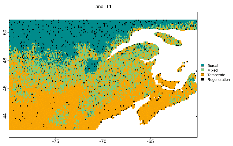
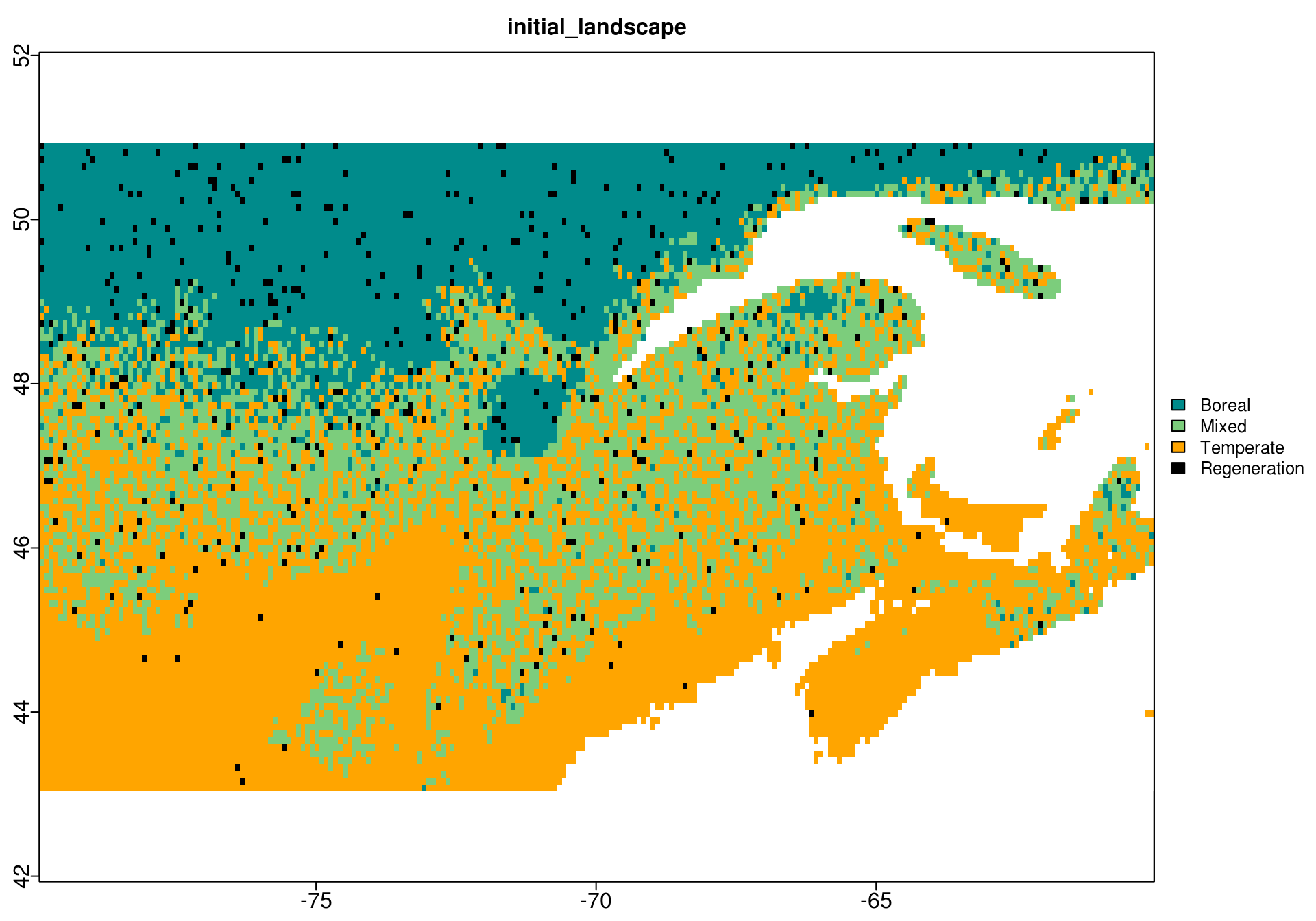
Let’s take a look in the initLand using the function plot_landscape():
plot_landscape(initLand, Title = 'initial_landscape')
Note that when using the real landscape the arguments xaxis, rmBorder and rangeLimitOccup are not considered.
Run the model
With the initial landscape set, we can now run the model using the function run_model(). We will run the model for 100 years (1 step = 5 years). For now the models supports only the RCP 8.5 scenario when using a real landscape:
lands <- run_model(steps = 20,
                   initLand = initLand)
The model output lands is a list containing a raster with all land steps and the initial climate condition (temperature and precipitation), and other useful information such as (i) steps, (ii) management intensity, (iII) RCP scenario and (v) landscape dimensions.
Plot output
For the real landscape you cannot use the functions plot_occupancy() and plot_rangeShift(), only animate().