Introduction

Climate warming poses a significant challenge for several species, particularly for trees that struggle to follow temperature warming and moving ranges (Sittaro et al. 2017). It is imperative to untangle the mechanisms governing their range limits to forecast how they will respond to climate change. The niche theory predicts that a species will be present in suitable environmental conditions that allow the species to have a positive growth rate (Hutchinson 1957). From this theory, we can define the geographic distribution of a species as a manifestation of individual demographic rates, such as growth, survival, and recruitment (Holt 2009). By assuming these demographic rates change with the environment, we can predict a species’ range limits based on its individuals’ performance (Maguire Jr 1973; Holt 2009).

Biotic interaction is undoubtedly an essential driver of demographic rates and, thereby, a potential driver of range limits. A recent theoretical framework based on coexistence theory has been proposed to assess how biotic interactions can scale up to affect range limits (Godsoe et al. 2017). Formally, this framework evaluates the intrinsic population growth rate when the focal species is rare (Chesson 2000), both in scenarios where there is no competition (fundamental niche) and when competitive species reach equilibrium (realized niche). Numerous studies have explored the influence of climate and competition on the distribution of forest trees across their ranges. For instance, Ettinger and HilleRisLambers (2017) observed in field experiments that neighboring competition constrained individual performance within the range but facilitated better performance outside the range. Using a dynamic forest model, Scherrer et al. (2020) showed how slow demographic rates and negative competition reduce the uphill migration rate of 16 tree species. Despite this evidence, the application of this framework to predict the geographic distribution of species based on demographic rates often reveals weak correlations between the performance of tree species and their distribution (McGill 2012; Thuiller et al. 2014; Csergo et al. 2017; Bohner and Diez 2020; Le Squin, Boulangeat, and Gravel 2021; Midolo, Wellstein, and Faurby 2021; Guyennon et al. 2023).

One possible explanation for such discrepancy between demographic rates and species distribution is the common practice of assessing performance under average conditions and pointwise estimations, neglecting the associated uncertainty in these estimates. In ecological models, the uncertainty in estimation arises from three distinct sources. The first source involves measurement errors, a factor often neglected in ecological models (Damgaard 2020). The second is process uncertainty linked to model (mis)specification (Harwood and Stokes 2003), determined by all variation that is not captured by the model covariates. Finally, even with a well-defined model and precise data, models must also consider parameter uncertainty due to individual variability (Cressie et al. 2009; Shoemaker et al. 2020).

Beyond data and model uncertainty, variability in demographic rates and subsequently in the population growth rate (\(\lambda\)) arises from two primary sources (van Daalen and Caswell 2020). The first is attributed to demographic and environmental stochasticity, where individuals exposed to identical conditions may exhibit different responses simply by chance (Caswell 2009). The second source of variability arises from heterogeneity encountered at various scales. These differences can manifest between individual stages that motivated the development of structured population models (Lewis 1942; Leslie 1945), and can promote high species diversity in forest trees (Clark 2010). Another source of heterogeneity arises from large-scale differences in neighboring patches, often described by the metapopulation theory (Levins 1969). This theory posits that the dynamics of occupied and empty patches in a landscape are driven by colonization and extinction processes. Building on this theory, Talluto et al. (2017) used patch variability to derive colonization and extinction rates of eastern North American trees, revealing their distribution to be out of equilibrium with climate. Therefore, while this result advances our understanding of the mechanisms governing large-scale tree distributions, there remains a need to reconcile it with local demographic dynamics, given that colonization and extinction processes ultimately manifest from demographic rates.

Theory predicts that the uncertainty arising from stochastic and heterogenous processes may lead to divergent outcomes in \(\lambda\). Demographic and environmental stochasticity may increase the uncertainty in \(\lambda\), consequently increasing the extinction risk, particularly for populations with low performance or low density (Holt et al. 2005; Gravel, Guichard, and Hochberg 2011). For instance, demographic stochasticity increased the extinction risk of European forest trees at the hot edge of their distribution (Guyennon et al. 2023). On the other hand, spatial heterogeneity has been described as a buffering process against the stochasticity in demographic rates, thereby increasing population persistence (Milles et al. 2023). This is particularly relevant in nonlinear models, where higher demographic and environmental stochasticity can increase the difference in population growth rate compared to the average expectations (Koons et al. 2009). Furthermore, demographic and environmental stochasticity influence abundance variation, indirectly impacting \(\lambda\) through density-dependence (May et al. 1978; Terry, O’Sullivan, and Rossberg 2022). A comprehensive understanding of the response of forest trees to climate change requires incorporating the multiple sources of variability arising from spatio-temporal variation and parameter uncertainty.

Here, we use a stochastic Integral Projection Model (IPM) to predict species-level intrinsic population growth (\(\lambda\)) for 31 eastern North American tree species. The IPM integrates the growth, survival, and recruitment demographic rates, which vary in response to climate and competition. By fitting each demographic rate using non-linear hierarchical Bayesian models, we capture parameter uncertainty at both the individual and local population scales. Additionally, our model naturally accommodates observed spatio-temporal stochasticity in climate and competition. Then, rather than ignoring these sources of variability, we embrace them into \(\lambda\) by defining species performance through a probabilistic framework. Specifically, we introduce a novel metric called local suitable probability, derived from the average population growth rate and its associated variability. This metric determines the probability of a positive population growth rate for a species under specific climate and competition conditions.

In our analysis, we first used the IPM to predict species-specific \(\lambda\) at the plot level under two conditions: without (fundamental niche) and with (realized niche) heterospecific competition. We replicated this calculation 100 times across all observed plots from the same species to assess the variability of \(\lambda\) arising from both spatio-temporal stochasticity in the climate and competition and model uncertainty. As this variable \(\lambda\) changes across space, we used these observations to model how the species’ local suitable probability changes across the mean annual temperature. Specifically, we ask how climate and competition affect each species’ local suitable probability. Then, we investigated how a species’ local suitable probability changes from the center of its distribution toward the cold and hot borders. Finally, we disentangle the relative impacts of climate and competition in changing suitable probability from the center to the borders. We conclude by discussing a novel theory that uses the local suitable probability to establish a link between individual demographic rates and metapopulation dynamics.

Methods

Population model, demographic components, and uncertainty structure

We use an Integral Projection Model (IPM) to predict the intrinsic population growth rate (\(\lambda\)) as a function of climate and competition. An IPM is a powerful modeling approach that allows a full representation of all sources of variability in demography. The IPM serves as a mathematical formulation describing the dynamics of a continuous trait distribution (\(z\)) within a population over discrete time steps:

\[ n(z', t + 1) = \int_{L}^{U} \, K(z', z, X, \theta)\, n(z, t)\, \mathrm{d}z \](1)

In our case, the trait \(z\) is defined as the tree’s diameter at breast height (dbh), constrained between the limits \(L\) and \(U\). The continuous distribution \(n(\cdot)\) of dbh \(z\) of a population at time \(t\) transitions to the next time step using a projection kernel (\(K\)). The kernel \(K\), with parameters \(\theta\) and covariates \(X\) that are time dependent, comprises three demographic submodels:

\[ K(z', z, \theta) = [Growth(z', z, X, \theta) \times Survival(z, X, \theta)] + Recruitment(z, X, \theta) \](2)

The growth model assesses the probability of an individual of size \(z\) at time \(t\) transitioning to size \(z'\) at time \(t+1\). The survival model determines the probability of an individual with size \(z\) at time \(t\) surviving to the next time step. Lastly, the recruitment model determines the number of new individuals entering the population at each time step as a function of total density \(z\). The kernel \(K\) has the same function of the population growth rate \(r\) in a population model, where multiplying the population distribution \(n(z, t)\) with \(K\) gives the population distribution at the next time step \(n(z', t+1)\). Its advantage in propagating uncertainty is that, instead of having a matrix with fixed parameters determining the transition rate of population individuals over time, it uses a probability distribution with uncertainty derived from the demographic models to project individuals over time.

With the defined \(K\), we can estimate the intrinsic population growth rate for a determined set of conditions from the covariates \(X\) and sampled parameters from the posterior distribution \(\theta\). Specifically, we discretize the continuous kernel \(K\) using the mid-point rule (Ellner, Childs, and Rees 2016) and estimate the intrinsic population growth rate using the dominant eigenvalue of the discretized \(K\). This approach is a local approximation of the population growth rate at the initial time steps.

A detailed description of the data and model development is available in Chapter 2. In summary, we evaluated non-linear statistical models to formulate the growth, survival, and recruitment components of the IPM, along with their uncertainty. Each demographic sub-model varies as a function of the mean annual temperature, mean annual precipitation, and stand basal area of larger individuals. Each model’s parameters (\(\theta\)) are species-specific, as each model is fitted separately for each species. Both climate variables influence each demographic model through an unimodal link function, where each model exhibits an optimal climate and niche breadth for temperature and precipitation. Additionally, density dependence is integrated based on the plot’s total basal area of larger individuals. Stand density affects growth and survival through a linear model, in which two parameters determine the strength of interaction from conspecific and heterospecific (all species combined) competition. For the recruitment model, the annual ingrowth rate is modulated by conspecific stand basal area, using an unimodal function to account for both the positive effect of seed source and the negative effect of conspecific competition. Furthermore, the annual survival rate of potential ingrowth individuals decreases linearly with the stand density of heterospecific individuals. Finally, the intercept of each growth, survival, and recruitment model incorporates plot-level random effects to control for the variance shared within the plot-year observations.

We use two open inventory datasets from eastern North America: the Forest Inventory and Analysis (FIA) dataset in the United States (O’Connell et al. 2007) and the permanent plots of forest inventory program for Québec (Minist‘ere des Ressources Naturelles 2016). These inventories, with multiple individual measurements over time and space, allowed us to use the transition information between measurement years for predicting growth, survival, and recruitment rates. We selected the 31 most abundant species, comprising 9 conifer species and 22 hardwood species, well-dispersed across shade tolerance and successional status (Supplementary Material 1). These species are well distributed across the eastern North American gradient and the sampling area covers cold and hot range limits for most species.

Extracting local suitability probability

We estimate \(\lambda\) at the local population scale, specifically at the plot level in our study. Within a given geographic location, such as a specific latitude where several plots are located, the variance of \(\lambda\) among those plots arises from spatio-temporal variations in both climate and competition covariates. For instance, climate stochasticity introduces noise in annual temperature and precipitation, leading to environmental variation. Similarly, even with identical climate conditions, two locations can exhibit different community abundance and composition, resulting in variability in the strength of competition. Beyond these spatio-temporal environmentally-induced variations, \(\lambda\) can still vary due to the other sources of uncertainty discussed above.

We track demographic model uncertainty at two complementary scales: individual and plot levels. At the individual level, without plot random effects, two plots with the same climate and competition conditions may have different \(\lambda\) values due to the uncertainty in the demographic growth, survival, and recruitment sub-models. Similarly, with the same environmental conditions and averaged parameter values (eliminating demographic uncertainty at the individual level), two plots can still yield different \(\lambda\) values due to the spatial uncertainty of each demographic model due to the plot random effects. Therefore, variability in the population growth rate can arise from spatio-temporal variations in both the environment and the parameters.

Given these different sources of variability in \(\lambda\), we define the suitable probability as the area under the distribution for \(\lambda \geq 1\). To estimate this, we first determine the cumulative distribution function, \(F(x)\), from the generic probability density function, \(\lambda = f(t)\), as follows:

\[ F_{\lambda}(x) = P(\lambda \le x) = \int_{-\infty}^{1} f(t)dt \](3)

This function represents the cumulative distribution from \(-\infty\) to \(x\). Subsequently, we define the suitable probability (\(\Lambda\)) as the complement of the cumulative distribution function for \(x = 1\):

\[ \Lambda = 1 - F_{\lambda}(1) \](4)

Modeling suitable probability

We can evaluate the suitable probability of a species at various scales, ranging from a single local plot up to several plots in a region. At the plot level, sources of variability in \(\lambda\) stem from parameter uncertainty, individual heterogeneity, and temporal variability in climate and competition. When considering multiple plots simultaneously, we can additionally account for spatial variability in climate and competition, along with spatial uncertainty in plot-level parameters.

Apart from parameter uncertainty at the individual level, all other sources of variability exhibit spatial dependence. This implies that environmental variability (from climate, competition, or both) and parameter uncertainty at the plot level can vary based on their spatial location. For instance, plots at the border of the species distribution may experience more temperature variability than those at the center. Additionally, plot-level parameter uncertainty can be spatially clustered, capturing potential features of demographic variability beyond the climatic and competition covariates, such as historical factors or local edaphic conditions.

Given that variability can be spatially dependent, we can model how suitable probability changes across the species’ range distribution, considering both fixed climate and competition effects and the underlying spatio-temporal variability. We are particularly interested in how suitable probability changes from the center toward the cold and hot ranges. For that, we categorized all species’ plot-year observations based on the gradient of mean annual temperature (MAT), divided into cold and hot ranges using the MAT centroid among all plots for the species (\(\frac{max(MAT) + min(MAT)}{2}\)). For instance, if a species is observed within the 4-10°C gradient of MAT, the plots with MAT below 7°C are classified as cold, while the others are classified as hot. We chose to use MAT instead of latitude because we are interested in the species’ climatic niche, although the two variables are highly correlated.

We assessed suitable probability separately for the cold and hot ranges, employing a linear model to determine the relationship between \(\lambda\) and MAT. The spatio-temporal variability of \(\lambda\) arising from environmental stochasticity and parameter uncertainty influences the variance of the linear model. As this variance may change depending on the range position, we introduce a submodel for the variance of the linear model to be dependent on MAT. To accommodate potential asymmetry in this variance, we use a Skew Normal Distribution (\(SN\)) incorporating an additional parameter (\(\alpha\)) that can introduce right or left-skewed tails to the variance:

\[ \begin{split} &log(\lambda) \sim SN(\xi, \omega, \alpha) \\[2pt] &\xi = \beta_{1, \xi} \times MAT + \beta_{0, \xi} \\[2pt] &\omega = e^{\beta_{1, \omega} \times MAT + \beta_{0, \omega}} \end{split} \](5)

Here, \(\xi\) is the location parameter or the \(\lambda\) average, and \(\omega\) is the scale representing the variance around the mean.

Simulations

We computed \(\lambda\) for each species based on the plot-year observations in the dataset, considering both environmentally induced variability and parameter uncertainty. For every observed species-plot-year combination, we incorporated temporal stochasticity in climate conditions by using the mean and standard deviation of mean annual temperature and precipitation calculated from the years between measurements. For instance, in the case of a plot observed twice, we calculated \(\lambda\) for the second observation with climate conditions drawn randomly from a normal distribution with mean and standard deviation extracted from plot specific climate observations for each year within the time interval. Similarly, temporal stochasticity in competition arises from variation in abundance and composition between measured years. By iteratively performing this calculation, drawing parameter values randomly from the posterior distribution, we introduced demographic uncertainty at the individual level. For each species-plot-year measurement, we replicated the calculation of \(\lambda\) 100 times. By applying this approach across all plots, we naturally incorporate spatial variation in climate and competition conditions and spatial uncertainty in plot-level parameters.

For each species-plot-year-replication combination, we calculated \(\lambda\) under two simulated conditions. The first scenario excludes competition in order to evaluate the fundamental niche, with heterospecific competition set at zero and conspecific total population size (N) set at 0.1. This simulation is used to assess the fundamental niche. The second scenario is used to evaluate the invasion growth rate with residents (the realized niche), with an evaluation of the population growth rate when the focal species is rare (\(N=0.1\)) and heterospecific competition is set to the observed abundance of the competitive species. This condition simulated the population growth rate under the realized niche.

We then fitted a linear model of \(\lambda\) for each species-plot-year-replication as a function of the mean annual temperature gradient. Species-specific linear models were evaluated for the hot and cold ranges using the Hamiltonian Monte Carlo (HMC) algorithm via the Stan software (version 2.30.1 Team and Others 2022) and the cmdstandr R package (version 0.5.3 Gabry, Češnovar, and Johnson 2023). We conducted 1000 iterations for the warm-up and 1000 iterations for the sampling phase for each of the four chains, resulting in 4000 posterior samples (excluding the warm-up). We used a sample of 5000 plots for each species to fit the model. This sample was necessary only for 6 out of the 31 species.

We leveraged the posterior distribution to estimate the suitable probability of a species for any value of MAT under fundamental or realized niches for the cold and hot ranges. Specifically, we estimated suitable probability under four different MAT conditions encountered by the species: at the border and the center of each cold and hot range. We defined the border of the cold range as the minimum observed MAT for the focal species in the dataset, while the hot range was defined as the maximum observed MAT. The center location is defined as the centroid of MAT for the focal species. Although the center location has the same MAT for the cold and hot ranges, both are retained because the model is fitted separately for the cold and hot ranges. Finally, we estimated suitable probability for each location under no competition (fundamental niche) and heterospecific competition (realized niche) conditions, using the empirical cumulative distribution function over 1000 predictive draws.

The code for the computation of each plot-year \(\lambda\) is available at https://github.com/willvieira/forest-IPM/tree/master/simulations/lambda_plot, and the code to model the linear model is at https://github.com/willvieira/forest-IPM/tree/master/simulations/model_lambdaPlot/.

Results

Model fit

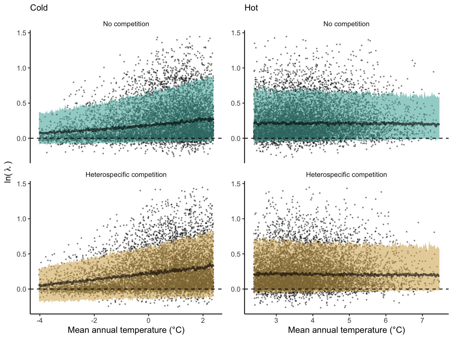
We first analyzed how the local population growth rate (\(\lambda\)) and its variability change across the cold and hot ranges (Equation 5). An example is provided at Figure 1 with the observed distribution of \(\lambda\) and the fit of the underlying model on the mean annual temperature gradient for balsam fir, Abies balsamea. Each point represents a plot-year-replication encompassing the complete spatio-temporal sources of variability arising from the stochastic environment and parameter uncertainty. The black line represents the fitted model of how \(\lambda\) changes with MAT, and the envelopes depict the 90th quantiles of model distribution. From this uncertainty, we can deduce the suitable probability. This example shows that the mean and variance of \(\lambda\) decrease towards the cold border, while it does not vary much towards the hot border. By comparing the model under heterospecific competition with that without competition for the cold range, we observed that while their average is similar, the uncertainty of the model under heterospecific competition shifted downwards (Figure 1, bottom left).

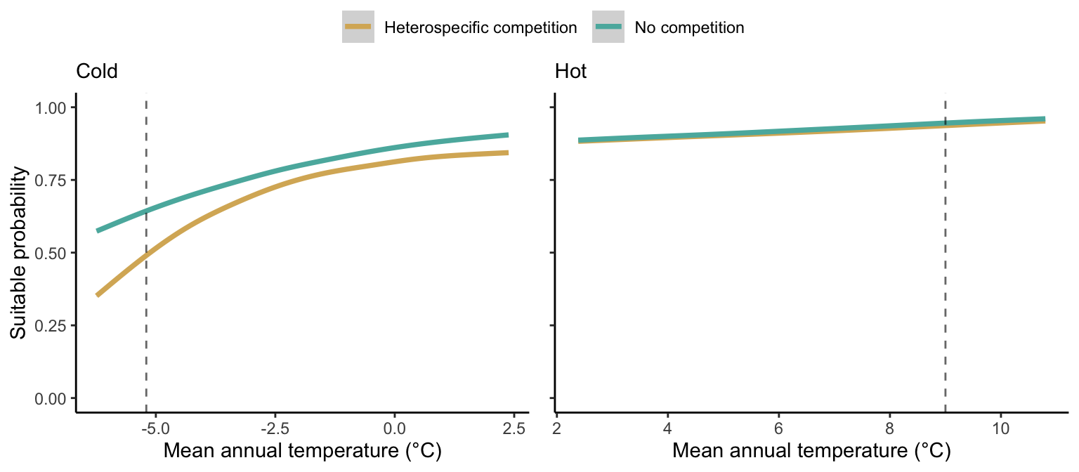
We then investigated the local suitability probability using the empirical cumulative distribution approach (Equation 4) from the linear model predictions. The Figure 2 shows the suitable probability expected over the mean annual temperature of the same species. We observed that the local suitability probability was reduced towards the cold border, with a stronger reduction under heterospecific competition (yellow curve). We can also observe that the decrease in suitable probability towards the border is nonlinear, becoming more substantial for heterospecific competition than for the no-competition condition.

The model fit and the estimation of suitable probability across the temperature gradient for all species are presented in Supplementary Material 2. We observed for most species a decrease of the climate effect at one border while the other remained unchanged. Additionally, a few species displayed a clear linear pattern of decreasing suitable probability from the cold to the hot border, with only one species (Betula papyrifera) having a decrease at both borders. Conversely, under the competition effect, most species exhibited a decrease in suitable probability at the hot border and an increase at the cold border, indicating a linear rise in the impact of competition from the cold to the hot border of the distribution.

Effect of climate and competition on suitable probability for the center and border distributions

We investigated the effect of climate and competition on the suitable probability at the border and center of the temperature range distribution for all species. Because the border and center positions are relative to each species, we could not represent the continuous trend in suitable probability across the MAT for all 31 species together. Instead, we extracted the local suitable probability with and without heterospecific competition for four locations across the MAT gradient (Figure 3). Overall, suitable probability was high among the species, with an average of 0.78. Among the four locations, species presented a lower suitable probability at the border of the hot range, with an average of 0.67. Across the temperature range, there is a monotonic decrease in suitable probability from the cold border toward the hot border.

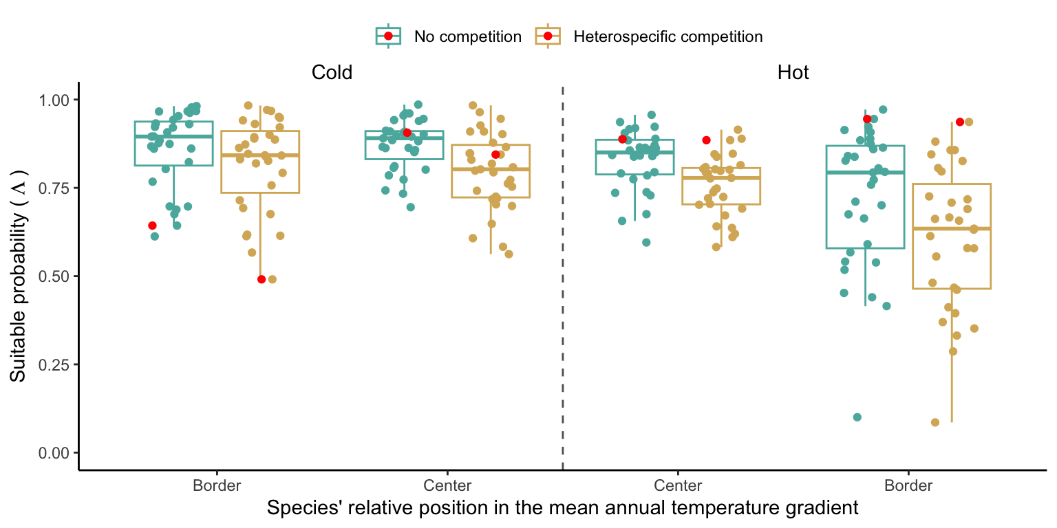
We further disentangle the influence of competition from that of climate by calculating the difference between suitable probability under heterospecific competition and without competition. A negative difference signifies competition reduces suitable probability, while positive differences indicate an increase. Across the four climate locations, heterospecific competition consistently reduced suitable probability for most species, with the magnitude of reduction intensifying from the cold to the hot border (Figure S1). This suggests that the decline in suitable probability observed from the cold to the hot border (Figure 3) results from the combined effect of climate and competition.

Suitable probability change from center to border

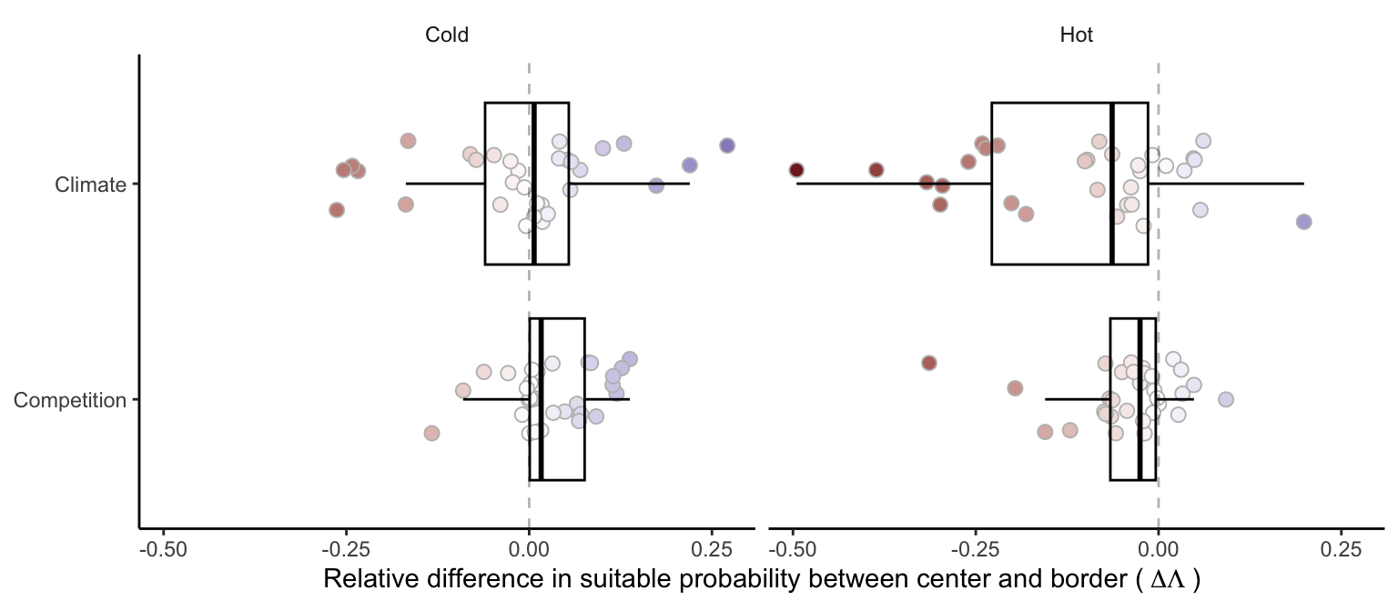
We investigated the relative effect of climate and competition on changing suitable probability from the center to the border of the species distribution (Figure 4). A positive relative difference indicates an increase in suitable probability from the center towards the border, while a negative difference indicates a decrease. Most species exhibited a decrease in suitable probability at the hot border relative to the center. Alternatively, most species showed a reduction in the effect of competition toward the cold border. However, the climate effect in the cold range was more variable, with some species experiencing an increase and others a decrease in suitable probability (Figure S2). Overall, the relative difference in suitable probability from the center toward the cold and hot borders was more influenced by climate rather than competition.

Discussion

Understanding the mechanisms shaping species distribution is imperative to face ongoing global changes. We acknowledged and integrated various sources of variability in the population growth rate of forest trees, contributing to an improved understanding of forest dynamics in an uncertain world. Introducing a novel metric, we quantified the relative impacts of climate and competition on the change in suitable probability across species distributions. Our findings revealed a nearly linear reduction in suitable probability from the cold to hot borders. Notably, the predominant influence on the relative difference in suitable probability from the center toward the border was attributed to climate rather than competition. These results, supported by a novel approach accounting for uncertainty, enhance our understanding of the nuanced interplay between climate and competition across species ranges.

The suitable probability was high across all species and range locations, with only around 5% of all species-location combinations having a suitable probability below the 0.5 threshold. This is primarily attributed to most species exhibiting a high positive population growth rate across their current range distribution. Additionally, the spatio-temporal variability in the environment and the parameter uncertainty in the plot may contribute to the elevated average population growth rate due to nonlinear averaging. This aligns with theoretical (Schreiber and Lloyd-Smith 2009) and empirical (Crone 2016) studies suggesting that spatial heterogeneity should increase the population growth rate.

Competition significantly reduces local suitability across all range locations, with a stronger and more consistent effect at the cold border, contributing to the ongoing debate surrounding its significance in setting range limits. Despite several studies emphasizing the effect of competition compared to climate on the demographic rates of forest trees (Zhang, Huang, and He 2015; Käber et al. 2021; Le Squin, Boulangeat, and Gravel 2021), debates persist regarding whether this effect at the local scale translates to the biogeographic distribution of species (Sober’on 2007; Copenhaver-Parry, Shuman, and Tinker 2017). Our findings support the Godsoe et al. (2017) hypothesis and a growing body of evidence (Scherrer et al. 2020; Shi et al. 2020; Paquette and Hargreaves 2021; Lyu and Alexander 2022) showing that the effect of competition on the intrinsic population growth rate can indeed contribute to range limits.

The decline in suitable probability from the cold to the hot border suggests a predominantly linear, rather than unimodal, relationship with temperature for most species (Figure S3). This result is consistent with reduced population growth rates in North American (Schultz et al. 2022; Le Squin, Boulangeat, and Gravel 2021) and European (Guyennon et al. 2023) forest trees, except for the contrasting pattern observation by Purves (2009). The higher suitable probability in the cold range compared to the hot range could be attributed to multiple factors. First, species may still follow their climate niche post the last glaciation, explaining why the current cold range limit does not align with the expected niche distribution (Svenning and Skov 2007), potentially leading to a colonization debt (Talluto et al. 2017). Notably, four of the six species exhibiting a significant decrease in suitable probability from the center toward the cold range were already at the extreme cold observed in the dataset (Figure S4).

Our model may however overlook crucial drivers of species performance, despite capturing a substantial amount of variation from parameter uncertainty at the plot level. Factors such as the impact of extreme temperature and precipitation on phenology can influence tree range limits (Morin, Augspurger, and Chuine 2007). Beyond covariates and plot-level uncertainty, incorporating temporal uncertainty at the plot level, accounting for spatio-temporal covariance, could likely capture additional sources of variation in demographic rates. While our approach considers temporal stochasticity in climate and competition, which affect species range size (Holt, Barfield, and Peniston 2022), there remains temporal variation in demographic rates beyond these covariates. This variability, possibly captured with random effects at the plot level, can influence range limits based on the degree of temporal autocorrelation and its relationship with the range (Benning, Hufbauer, and Weiss-Lehman 2022). For instance, an empirical study on perennial herbaceous species demonstrated that temporal environmental stochasticity reduced the population growth rate relative to the average (Crone 2016). In our study, this temporal variability is particularly relevant for survival (due to disturbance) and recruitment (due to phenology) rates because, in addition to having high temporal variability (Clark et al. 1999; de Souza Leite et al. 2023), they represent the most significant drivers of population growth rate (Chapter 2).

The effect of competition, similar to climate, increased from the center towards the border of the hot range, contrary to Kunstler et al. (2021), who found no difference in the competition effect between the center and border of the species. Additionally, our results deviate from the Species Interactions-Abiotic Stress Hypothesis, predicting a stronger competition effect in less stressful climate conditions (Louthan, Doak, and Angert 2015). When considering the relative position of the species across the temperature gradient, only the effect of climate at the cold range changed with temperature. This indicates that most species have a similar or higher suitable probability at the border of the cold range compared to their center distribution. We further tested whether the species’ range size affects the relative difference in suitable probability; while the absolute values change, the pattern among the species remains unchanged.

The climate gradient of temperature had a more significant effect than competition in changing the suitable probability of forest trees. This means that mean annual temperature, along with all latent variables, better explains how suitable probability changes across the temperature range. The choice of using only mean annual temperature as an explanatory variable for the variance of \(\lambda\) can be improved. For instance, the model could be built accounting for mean annual temperature and precipitation to predict the complete two-dimensional distribution of the species’ climate niche. Plot random effects could be further used to account for the nestedness of the data design, allowing the proper separation of the total variance of the metamodel into variance arising from individual- and plot-level demographic uncertainty. While we have assumed climate variability as independent and identically distributed random variables, this assumption can be relaxed to include temporal autocorrelation. Autocorrelated environmental fluctuation can significantly change a species’ range limits due to nonlinear averaging (Benning, Hufbauer, and Weiss-Lehman 2022; Holt, Barfield, and Peniston 2022). Lastly, although coexistence theory assumes the abundance of competitors to be at equilibrium (Chesson 2000), testing this assumption remains practically impossible.

Despite the many ways of improving our study, there is a growing body of evidence indicating a mismatch between performance and occurrence (McGill 2012; Thuiller et al. 2014; Csergo et al. 2017; Bohner and Diez 2020; Le Squin, Boulangeat, and Gravel 2021; Midolo, Wellstein, and Faurby 2021; Guyennon et al. 2023). Our approach can better capture the nuanced effect of climate and competition along with the spatio-temporal variation in \(\lambda\), yet it was not enough to fully predict tree range limits. Since species distribution is influenced by processes at multiple scales (McGill 2010; Heffernan et al. 2014), it is challenging to rely on a single individual-level performance metric to predict it all (Evans et al. 2016). For instance, dispersion plays a crucial role in changing species distribution at larger spatial scales, either reducing its extent due to limited dispersal or increasing it through source-sink dynamics (Pulliam 2000). We propose that our novel metric, local suitable probability, can be a key unifying factor linking local and landscape scales.

Forest trees exhibit variation in their frequency of occurrence across distribution gradients, yet their relative abundance remains consistent when present (Canham and Thomas 2010). Such observation implies that assessing forest distribution should focus on colonization and extinction patch dynamics rather than local performance (Canham and Murphy 2017). However, instead of restricting models to either local or large scales, we propose using the local suitable probability to reconcile the local demographic dynamics with the metapopulation theory. Colonization and extinction processes, as described by metapopulation theory (Levins 1969), are well-suited for describing the mosaic of forest successional stages at the landscape scale resulting from natural disturbances and succession. However, an implicit assumption is that unoccupied patches are necessarily available for colonization. We relax this assumption and quantify patch availability using the local suitable probability metric (\(\Lambda\)). Considering an ensemble of patches (\(p\)) where individuals can arrive and establish in empty patches through colonization (\(\alpha\)), and occupied patches can become empty through extinction (\(\varepsilon\)), the integrated metapopulation model becomes:

\[ \frac{dp}{dt} = \alpha p (\Lambda - p) - \varepsilon p \](6)

With this formulation, rather than having \(1 - p\) available patches for colonization, we have \(\Lambda - p\). Therefore, when \(\lambda\) and its variability are high, the local suitable probability equals 1, indicating that all non-occupied patches are available. Conversely, as the local suitable probability decreases, the proportion of non-occupied patches available for colonization is reduced. This integrative approach allows one to account for both the local (e.g. competition and climate) and landscape (e.g. fire disturbances and dispersal) drivers of forest dynamics when assessing tree distribution.

References

Benning, John W., Ruth A. Hufbauer, and Christopher Weiss-Lehman. 2022. “Increasing temporal variance leads to stable species range limits.” Proceedings of the Royal Society B: Biological Sciences 289 (1974). https://doi.org/10.1098/rspb.2022.0202.
Bohner, Teresa, and Jeffrey Diez. 2020. “Extensive mismatches between species distributions and performance and their relationship to functional traits.” Ecology Letters 23 (1): 33–44.
Canham, Charles D., and Lora Murphy. 2017. “The demography of tree species response to climate: Sapling and canopy tree survival.” Ecosphere 8 (2). https://doi.org/10.1002/ecs2.1701.
Canham, Charles D, and R Quinn Thomas. 2010. “Frequncy, not relative abundance, of temperate tree species varies along climate gradients in eastern North America.” Ecology 91 (12): 3433–40. https://doi.org/10.1890/10-0312.1.
Caswell, Hal. 2009. “Stage, age and individual stochasticity in demography.” Oikos 118 (12): 1763–82. https://doi.org/https://doi.org/10.1111/j.1600-0706.2009.17620.x.
Chesson, Peter. 2000. “Mechanisms of maintenance of species diversity.” Annu. Rev. Ecol. Syst 31: 343–66. https://doi.org/10.1146/annurev.ecolsys.31.1.343.
Clark, James S. 2010. “Individuals and the variation needed for high species diversity in forest trees.” Science 327 (5969): 1129–32. https://doi.org/10.1126/science.1183506.
Clark, J. S., B. Beckage, P. Camill, B. Cleveland, J. HilleRisLambers, J. Lichter, J. McLachlan, J. Mohan, and P. Wyckoff. 1999. “Interpreting recruitment limitation in forests.” American Journal of Botany 86 (1): 1–16. https://doi.org/10.2307/2656950.
Copenhaver-Parry, Paige E., Bryan N. Shuman, and Daniel B. Tinker. 2017. “Toward an improved conceptual understanding of North American tree species distributions.” Ecosphere 8 (6): e01853. https://doi.org/10.1002/ecs2.1853.
Cressie, Noel, Catherine A. Calder, James S. Clark, Jay M. Ver Hoef, and Christopher K. Wikle. 2009. “Accounting for uncertainty in ecological analysis: The strengths and limitations of hierarchical statistical modeling.” Ecological Applications 19 (3): 553–70. https://doi.org/10.1890/07-0744.1.
Crone, Elizabeth E. 2016. “Contrasting effects of spatial heterogeneity and environmental stochasticity on population dynamics of a perennial wildflower.” Journal of Ecology 104 (2): 281–91. https://doi.org/10.1111/1365-2745.12500.
Csergo, Anna M., Roberto Salguero-G’omez, Olivier Broennimann, Shaun R. Coutts, Antoine Guisan, Amy L. Angert, Erik Welk, et al. 2017. “Less favourable climates constrain demographic strategies in plants.” Ecology Letters. https://doi.org/10.1111/ele.12794.
Damgaard, Christian. 2020. “Measurement Uncertainty in Ecological and Environmental Models.” Trends in Ecology and Evolution 35 (10): 871–73. https://doi.org/10.1016/j.tree.2020.07.003.
de Souza Leite, Melina, Sean M. McMahon, Paulo In’acio Prado, Stuart J. Davies, Alexandre Adalardo de Oliveira, Hannes P. De Deurwaerder, Salom’on Aguilar, et al. 2023. “Major axes of variation in tree demography across global forests.” bioRxiv. https://www.biorxiv.org/content/10.1101/2023.01.11.523538v2.abstract.
Ellner, Stephen P, Dylan Z Childs, and Mark Rees. 2016. Data-driven modelling of structured populations. Springer.
Ettinger, Ailene, and Janneke HilleRisLambers. 2017. “Competition and facilitation may lead to asymmetric range shift dynamics with climate change.” Global Change Biology 23 (9): 3921–33. https://doi.org/10.1111/gcb.13649.
Evans, Margaret E K, Cory Merow, Sydne Record, Sean M. McMahon, and Brian J. Enquist. 2016. “Towards Process-based Range Modeling of Many Species.” Trends in Ecology and Evolution 31 (11): 860–71. https://doi.org/10.1016/j.tree.2016.08.005.
Gabry, Jonah, Rok Češnovar, and Andrew Johnson. 2023. cmdstanr: R Interface to ’CmdStan’.
Godsoe, William, Jill Jankowski, Robert D Holt, and Dominique Gravel. 2017. “Integrating Biogeography with Contemporary Niche Theory.” Trends in Ecology and Evolution 32 (7): 488–99. https://doi.org/10.1016/j.tree.2017.03.008.
Gravel, Dominique, Fr’ed’eric Guichard, and Michael E Hochberg. 2011. “Species coexistence in a variable world.” Ecology Letters 14 (8): 828–39. https://doi.org/10.1111/j.1461-0248.2011.01643.x.
Guyennon, Arnaud, Björn Reineking, Roberto Salguero-Gomez, Jonas Dahlgren, Aleksi Lehtonen, Sophia Ratcliffe, Paloma Ruiz-Benito, Miguel A Zavala, and Georges Kunstler. 2023. “Beyond mean fitness: Demographic stochasticity and resilience matter at tree species climatic edges.” Global Ecology and Biogeography 32 (4): 573–85. https://doi.org/https://doi.org/10.1111/geb.13640.
Harwood, John, and Kevin Stokes. 2003. “Coping with uncertainty in ecological advice: Lessons from fisheries.” Trends in Ecology and Evolution 18 (12): 617–22. https://doi.org/10.1016/j.tree.2003.08.001.
Heffernan, James B, Patricia A Soranno, Michael J Angilletta, Lauren B Buckley, Daniel S Gruner, Tim H Keitt, James R Kellner, John S Kominoski, Adrian V Rocha, and Jingfeng Xiao. 2014. “Macrosystems ecology: understanding ecological patterns and processes at continental scales.” Frontiers in Ecology and the Environment 12 (1): 5–14.
Holt, Robert D. 2009. “Bringing the Hutchinsonian niche into the 21st century: ecological and evolutionary perspectives.” Proceedings of the National Academy of Sciences 106 (supplement_2): 19659–65.
Holt, Robert D., Michael Barfield, and James H. Peniston. 2022. “Temporal variation may have diverse impacts on range limits.” Philosophical Transactions of the Royal Society B: Biological Sciences 377 (1848). https://doi.org/10.1098/rstb.2021.0016.
Holt, Robert D, Timothy H Keitt, Mark a Lewis, Brian a Maurer, and Mark L Taper. 2005. “Theoretical models of species’ borders: single species approaches.” Schurr2012 108 (1): 18–27. https://doi.org/10.1111/j.0030-1299.2005.13147.x.
Hutchinson, G Evelyn. 1957. “Concluding remarks.” In Cold Spring Harbor Symposium on Quantitative Biology, 22:415–27.
Käber, Yannek, Peter Meyer, Jonas Stillhard, Emiel De Lombaerde, Jürgen Zell, Golo Stadelmann, Harald Bugmann, and Christof Bigler. 2021. “Tree recruitment is determined by stand structure and shade tolerance with uncertain role of climate and water relations.” Ecology and Evolution 11 (17): 12182–12203. https://doi.org/10.1002/ece3.7984.
Koons, David N, Samuel Pavard, Annette Baudisch, and C Jessica E. Metcalf. 2009. “Is life-history buffering or lability adaptive in stochastic environments?” Oikos 118 (7): 972–80. https://doi.org/https://doi.org/10.1111/j.1600-0706.2009.16399.x.
Kunstler, Georges, Arnaud Guyennon, Sophia Ratcliffe, Nadja Rüger, Paloma Ruiz-Benito, Dylan Z. Childs, Jonas Dahlgren, et al. 2021. “Demographic performance of European tree species at their hot and cold climatic edges.” Journal of Ecology 109 (2): 1041–54. https://doi.org/10.1111/1365-2745.13533.
Leslie, Patrick H. 1945. “On the use of matrices in certain population mathematics.” Sankhyt 33 (3): 183–212.
Le Squin, Amaël, Isabelle Boulangeat, and Dominique Gravel. 2021. “Climate-induced variation in the demography of 14 tree species is not sufficient to explain their distribution in eastern North America.” Global Ecology and Biogeography 30 (2): 352–69. https://doi.org/10.1111/geb.13209.
Levins, Richard. 1969. “Some Demographic and Genetic Consequences of Environmental Heterogeneity for Biological Control.” Bulletin of the Entomological Society of America 15 (3): 237–40. https://doi.org/10.1093/besa/15.3.237.
Lewis, E G. 1942. “On the generation and growth of a population.” Sankhyã 6: 93–96.
Louthan, Allison M., Daniel F. Doak, and Amy L. Angert. 2015. “Where and When do Species Interactions Set Range Limits?” Trends in Ecology and Evolution 30 (12): 780–92. https://doi.org/10.1016/j.tree.2015.09.011.
Lyu, Shengman, and Jake M. Alexander. 2022. “Competition contributes to both warm and cool range edges.” Nature Communications 13 (1): 1–9. https://doi.org/10.1038/s41467-022-30013-3.
Maguire Jr, Bassett. 1973. “Niche response structure and the analytical potentials of its relationship to the habitat.” The American Naturalist 107 (954): 213–46.
May, Robert M, J R Beddington, J W Horwood, and J G Shepherd. 1978. “Exploiting natural populations in an uncertain world.” Mathematical Biosciences 42 (3-4): 219–52.
McGill, Brian J. 2010. “Matters of scale.” Science 328 (5978): 575–76. https://doi.org/10.1126/science.1188528.
———. 2012. “Trees are rarely most abundant where they grow best.” Journal of Plant Ecology 5 (1): 46–51. https://doi.org/10.1093/jpe/rtr036.
Midolo, Gabriele, Camilla Wellstein, and Søren Faurby. 2021. “Individual fitness is decoupled from coarse-scale probability of occurrence in North American trees.” Ecography 44 (5): 789–801. https://doi.org/https://doi.org/10.1111/ecog.05446.
Milles, Alexander, Thomas Banitz, Milos Bielcik, Karin Frank, Cara A Gallagher, Florian Jeltsch, Jane Uhd Jepsen, Daniel Oro, Viktoriia Radchuk, and Volker Grimm. 2023. “Local buffer mechanisms for population persistence.” Trends in Ecology & Evolution 38 (13): 1051–9.
Minist‘ere des Ressources Naturelles. 2016. “Norme d’inventaire ecoforestier: placettes-echantillons temporaires.” Direction des inventaires forestier, Ministère des Ressources naturelles,Québec.
Morin, Xavier, Carol Augspurger, and Isabelle Chuine. 2007. “Process-based modeling of species’ distributions: what limits temperate tree species’ range boundaries?” Ecology 88 (9): 2280–91. https://doi.org/10.1890/06-1591.1.
O’Connell, M B, E B LaPoint, J A Turner, T Ridley, D Boyer, A Wilson, K L Waddell, and B L Conkling. 2007. “The forest inventory and analysis database: Database description and users forest inventory and analysis program.” US Department of Agriculture, Forest Service.
Paquette, Alexandra, and Anna L Hargreaves. 2021. “Biotic interactions are more often important at species’ warm versus cool range edges.” Ecology Letters 24 (11): 2427–38. https://doi.org/https://doi.org/10.1111/ele.13864.
Pulliam, H. Ronald. 2000. “On the relationship between niche and distribution.” Ecology Letters 3 (4): 349–61. https://doi.org/10.1046/j.1461-0248.2000.00143.x.
Purves, Drew W. 2009. “The demography of range boundaries versus range cores in eastern US tree species.” Proceedings of the Royal Society B: Biological Sciences 276 (1661): 1477–84. https://doi.org/10.1098/rspb.2008.1241.
Scherrer, Daniel, Yann Vitasse, Antoine Guisan, Thomas Wohlgemuth, and Heike Lischke. 2020. “Competition and demography rather than dispersal limitation slow down upward shifts of trees’ upper elevation limits in the Alps.” Journal of Ecology, no. March: 1–15. https://doi.org/10.1111/1365-2745.13451.
Schreiber, Sebastian J., and James O. Lloyd-Smith. 2009. “Invasion dynamics in spatially heterogeneous environments.” American Naturalist 174 (4): 490–505. https://doi.org/10.1086/605405.
Schultz, Emily L, Lisa Hülsmann, Michiel D Pillet, Florian Hartig, David D Breshears, Sydne Record, John D Shaw, R Justin DeRose, Pieter A Zuidema, and Margaret E K Evans. 2022. “Climate-driven, but dynamic and complex? A reconciliation of competing hypotheses for species’ distributions.” Ecology Letters 25 (1): 38–51.
Shi, Hang, Quan Zhou, Fenglin Xie, Nianjun He, Rui He, Kerong Zhang, Quanfa Zhang, and Haishan Dang. 2020. “Disparity in elevational shifts of upper species limits in response to recent climate warming in the Qinling Mountains, North-central China.” Science of the Total Environment 706: 135718. https://doi.org/10.1016/j.scitotenv.2019.135718.
Shoemaker, Lauren G., Lauren L. Sullivan, Ian Donohue, Juliano S. Cabral, Ryan J. Williams, Margaret M. Mayfield, Jonathan M. Chase, et al. 2020. “Integrating the underlying structure of stochasticity into community ecology.” Ecology 101 (2): 1–15. https://doi.org/10.1002/ecy.2922.
Sittaro, Fabian, Alain Paquette, Christian Messier, and Charles A. Nock. 2017. “Tree range expansion in eastern North America fails to keep pace with climate warming at northern range limits.” Global Change Biology, 1–10. https://doi.org/10.1111/gcb.13622.
Sober’on, Jorge. 2007. “Grinnellian and Eltonian niches and geographic distributions of species.” Ecology Letters 10 (12): 1115–23. https://doi.org/10.1111/j.1461-0248.2007.01107.x.
Svenning, Jens Christian, and Flemming Skov. 2007. “Could the tree diversity pattern in Europe be generated by postglacial dispersal limitation?” Ecology Letters 10 (6): 453–60. https://doi.org/10.1111/j.1461-0248.2007.01038.x.
Talluto, Matthew V., Isabelle Boulangeat, Steve Vissault, Wilfried Thuiller, and Dominique Gravel. 2017. “Extinction debt and colonization credit delay range shifts of eastern North American trees.” Nature Ecology & Evolution 1 (June): 0182. https://doi.org/10.1038/s41559-017-0182.
Team, Stan Development, and Others. 2022. “Stan modeling language users guide and reference manual, version 2.30.1.” Stan Development Team.
Terry, J Christopher D, Jacob D O’Sullivan, and Axel G Rossberg. 2022. “Synthesising the multiple impacts of climatic variability on community responses to climate change.” Ecography 2022 (5): e06123.
Thuiller, Wilfried, Tamara Munkemuller, Katja H Schiffers, Damien Georges, Stefan Dullinger, Vincent M Eckhart, Thomas C Edwards, et al. 2014. “Does probability of occurrence relate to population dynamics?” Ecography 37 (12): 1155–66. https://doi.org/10.1111/ecog.00836.
van Daalen, Silke, and Hal Caswell. 2020. “Variance as a life history outcome: Sensitivity analysis of the contributions of stochasticity and heterogeneity.” Ecological Modelling 417 (108856).
Zhang, Jian, Shongming Huang, and Fangliang He. 2015. “Half-century evidence from western Canada shows forest dynamics are primarily driven by competition followed by climate.” Proceedings of the National Academy of Sciences 112 (13): 4009–14. https://doi.org/10.1073/pnas.1420844112.